I like taking logs, but sometimes you can’t, because the data have zeroes. So sometimes I’ll take the square root (as, for example for the graphs on the cover of our book). But often the square root doesn’t seem to go far enough. Also it lacks the direct interpretation of the log. Peter Hoff told me that Besag prefers the 1/4-power. This seems like it might make sense in practice, although I don’t really have a good way of thinking about it–except maybe to think that if the dynamic range of the data isn’t too large, it’s pretty much like taking the log. But then why not the 1/8 power? Maybe then you get weird effects near zero? I haven’t ever really seen a convincing treatment of this problem, but I suspect there’s some clever argument that would yield some insight.
Here’s my first try: a set of plots of various powers (1/8, 1/4, 1/2, and 1, i.e., eighth-root, fourth-root, square-root, and linear), each plotted along with the logarithm, from 0 to 50:
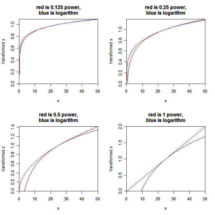
OK, here’s the point. Suppose you have data that mostly fall in the range [10, 50]. then the 1/4 power (or the 1/8 power) is a close fit to the log, which means that the coefficients in a linear model on the 1/4 power or the 1/8 power can be interpreted as muliplicative effects.
On this scale, the difference between either of these powers and the log occurs at the low end of the scale. As x goes to 0, the log actually goes to negative infinity, and the powers go to zero. The big difference betwen the 1/8 power and the 1/4 power is that the x-points near 0 are mapped much further away from the rest for the 1/4 power than for the 1/8 power.
An argument in favor of the 1/4-power transformation thus goes as follows:
First, the 1/4 power maps closely to the log over a reasonably large range of data (a factor of 5, for example from 10 to 50). Thus, an additive model on the 1/4-power scale approximately corresponds to a multiplicative model, which is typically what we want. (In contrast, the square-root does not map so well, and so a model on that scale is tougher to interpret.)
Second, on the 1/4-power scale, the x-points near zero map reasonably close to the main body of points. So we’re not too worried about these values being unduly influential in our analysis. (In contrast, the 1/8-power takes x=0 and puts it so far away from the other data that I could imagine it messing up the model.)
Could this argument be made more formally? I’ve never actually used the 1/4 power, but I’m wondering if maybe it really is a good idea.
P.S. Just to clear up a few things: the purpose of a transformation, as I see it, is to get a better fit and better interpretability for an additive model. Students often are taught that transformations are about normality, or about equal variance, but these are chump change compared to additivity and interpretability.
I remember reading somewhere someone advocating adding a small number (with what counts as small presumably depending on the range of the data) to either (a) just the zero values or (b) all data points in the sample, as an alternative way of getting around this. Do you have any thoughts on this?
Conchis,
Yes, I've seen the transformation g(x) = log(c+x), which indeed is close to the log for x>>c. The key seems to be choosing a reasonable value of c. If it's too small, then it can make zeroes into outliers on the transformed scale (as with the 1/8 power, above). The funny thing is that I usually see c picked completely arbitrarily. For example, x is income in dollars, and c=1. Or x is income in thousands of dollars, and c=1. There's gotta be some underlying model here to which this is a reasonable approximation; just picking c=1 can't be a good general strategy!
So, yeah, I think that in the paper that clears up this issue, both the power transformation and the log(c+x) transformation should be considered.
I do not understand your graphs. Does the log depend on the power? Why is the log curve different in each case? It seens that the log of 27 is 1 in each case, but the number whose log is .5 seems to vary a lot.
Thanks,
Jim
P.S. I have learned a lot from this blog over the years. Pleawse keep up the good work.
Jim,
Yes, the curves are rescaled in each case to line up and match first derivatives at the middle of the range. Also, the logs go to negative infinity, but I cut the y-scale off at 0.
I suggest you edit "the fourth power (or the eighth power) is a close fit to the log". You mean "quarter power" or "one-fourth power".
Roger,
Thanks.
From an email conversation I just had with Julian Besag:
“The reasoning (for the quarter power transformation) back in the late 70's was mainly empirical. I had learnt about EDA at Princeton in 1975 from John Tukey and
imported it to the UK and Durham Univ in particular. The quarter
power often seemed to be successful in stabilizing variance and
in producing approx additivity (esp in 2-way tables, for which
I'd written a simple program for identifying the power, based
on JT's 1dfr for non-additivity). Allan Seheult and I coined
the term "the Durham law" for the quarter power. JT concentrated
on sqroots, logs and inverses.''
"I think that in the paper that clears up this issue, both the power transformation and the log(c+x) transformation should be considered." I'd like to read that paper.
Adding a constant does seem to have been studied for some situations such as odds ratios for 2×2 tables. It seems intuitively more appropriate in those cases (assuming c is between 0 and 1) on the basis that the true probability of occurance is deemed a priori not to be zero for cells with zero counts. I think that adding c = 0.5 is attributed to JBS Haldane (and the resulting odds ratio known as the Haldane estimator in some circles).
My intution is the effects of the approaches might be different in testing and prediction, but i haven't thought it through.
Thom
Tukey wrote a nice paper on the topology of transformations:
On the Comparative Anatomy of Transformations
John W. Tukey
The Annals of Mathematical Statistics, Vol. 28, No. 3. (Sep., 1957), pp. 602-632.
For what it is worth, The book "Statistics for Experimenters", Box, Hunter & Hunter, has a very extensive discussion of transformations.
Kjetil
Andrew,
Jim did not understand your graphs, and even with your explanation, I do not still understand.
For example, on the "0.5 power" graph, square root of 50 has never been equal to 1.4 … and Log(25) has never been equal to 1 …
Can you explain or more simply give your R-code ?
Thanks
plotcurves