Last month I posted an article on the sister blog: How much does advertising matter in presidential elections?, discussing a paper by Brett Gordon and Wesley Hartmann.

Gordon sent in an update:

Both Wes and I greatly appreciate your comments and for highlighting our work. All the points you raise are quite fair. As you might have guessed, similar issues arose during the review process. Below we’d just like to briefly elaborate on three of your points.

1) As you note, candidates’ marketing activities are not limited to TV advertising. We think the big question is the sign of the bias. In OLS, it’s true that if other types of advertising are positively correlated with TV advertising, our estimate would be an upper bound. Our primary specification is 2SLS, which might have a different bias arising from the potentially problematic correlation between TV ad prices (our first-stage instrumental variables) and these other marketing activities. Because TV ad prices drive down observed advertising, but might increase other marketing activities, it seems that high TV ad prices would not reduce votes as much as they should, leading to an underestimate. Potential correlations between ad prices and the costs of these other instruments could, however, start to shift the bias back in the positive direction as you suggest. It’s not clear, at least to us, how this bias would eventually play out.

Needless to say, it would be great to integrate additional measures of campaign marketing activities in order to tease out their relative effects. But of course, this introduces additional endogenous variables, which would require additional instrumental variables. We decided to leave this to future work.

2) We completely agree that advertising effects are likely heterogeneous, such that there is some unobservable at the market (or perhaps county) level that interacts with our advertising variable. A savvy campaigner might observe this variable, or at the least, have some belief over its possible values.

We experimented with a couple approaches to deal with this. For instance, we tried interacting the advertising variable with the percentage of self-identified independents in a market, with the thought that these types of voters might be more responsive to advertising. We also tried including a random effect directly on the advertising coefficient. However, neither approach was successful in recovering any significant heterogeneity. We think the issue is simply that our voting outcomes lack sufficient variation once we’ve conditioned on the various controls and fixed effects. (That is, if we omit many of the controls, especially the DMA-party fixed effects, we do obtain a positive estimate of the standard deviation on the random effect.)

Note that we use 2SLS to deal with the endogeneity of the advertising variables. If the unobservable interaction is at the market level, and one believes our instrumental variables assumptions, then Wooldridge (Economic Letters, 1997) shows 2SLS yields consistent estimates of the coefficient on the endogenous variable despite the presence of such unobservables. We discuss this in the paper in section 3.2 on page 29.

With all of that said, the fact that we do not recover heterogeneity in the advertising coefficient obviously doesn’t imply there is no such heterogeneity. We simply seem unable to estimate heterogeneous effects with our particular data set.

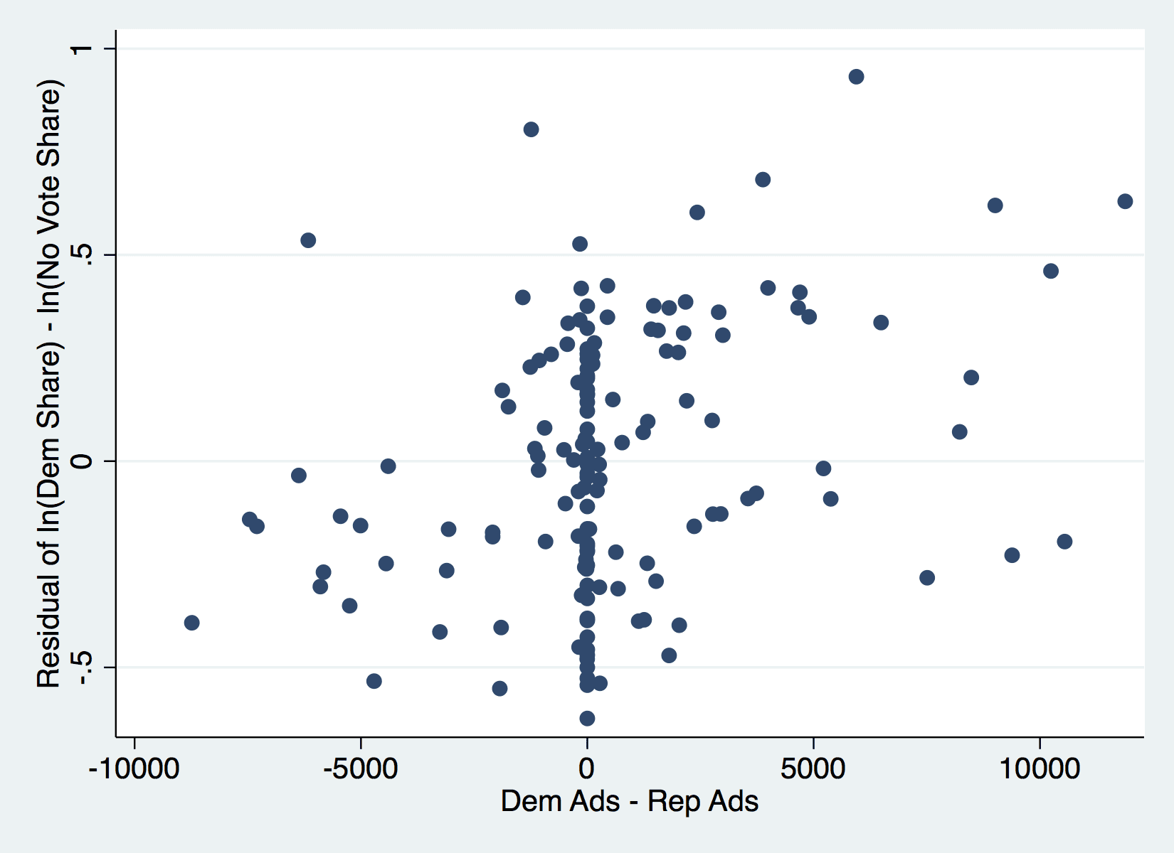
3) Thanks for raising the last point about a plot. Here is a plot that is very close to what you requested, for reasons I’ll explain next.

In addition to the market-level Republican and Democratic vote shares, there is the share of voters who chose not to vote at all. Focusing on the relative Democratic and Republican vote shares misses variation in the turnout rate. An increase in advertising by both candidates could increase turnout without changing the relative shares. For this reason, the dependent variable in the regression is:

ln(democrat’s vote share) – ln(no vote share)

As you suggested, everything is now at the market level. I obtain the residuals from this first-stage regression excluding advertising, but including the fixed effects and controls. The x-axis is the difference between Democratic and Republican advertising in the market. A simple regression of the residuals against the difference in ad levels yields a small positive coefficient with a t-stat of 3.8 (calculated using robust SEs).

Just in case you’re interested, Wes and I have another paper that focuses more on modeling the behavior of the candidates.

The primary focus of this paper is to examine how candidates’ TV advertising strategies would have changed under a direct voting system, instead of the Electoral College.