I keep pointing people to this article by Carl Morris so I thought I’d post it. The article is really hard to find because it has no title: it appeared in the Journal of the American Statistical Association as a discussion of a couple of other papers.
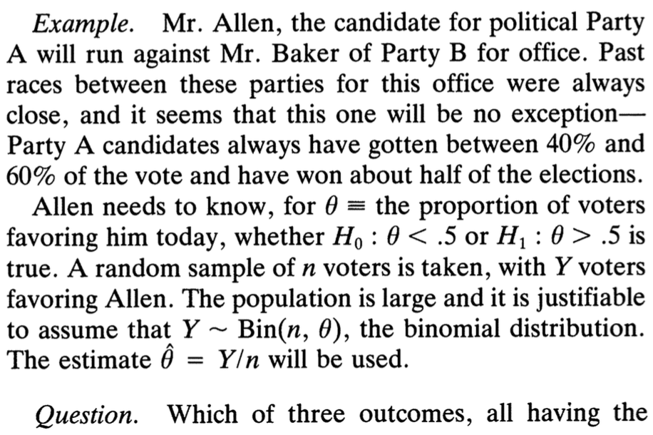
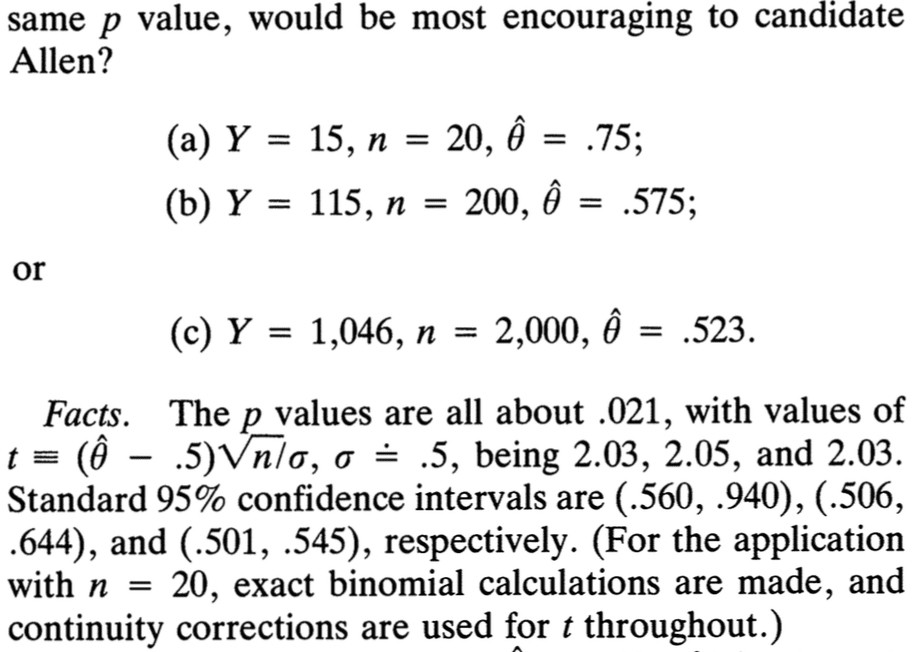
All 3 scenarios have the same p-value. And, given the way that statistics is typically taught (slogans about “statistical significance” vs. “practical significance”), one might think that scenario (a) is the best for the candidate, as the estimate is the largest in scenario A above.
Think about it: a higher estimate is good for Mr. Allen, and a smaller p-value is good for Mr. Allen. So it stands to reason that, with equal p-values, the larger estimate will be the better news.
And look at the 95% confidence intervals:
A: (.560, .940)
B: (.506, .644)
C: (.501, .545)
A looks best, no? The decision doesn’t even seem close.
But, no, as Carl explains, scenario C is the most encouraging for Mr. Allen.
Regular readers of this blog will recognize scenario A as the noisy-data situation where statistical significance tells you very little:
It might get you a publication in Psychological Science or the tabloids but that’s about it.
This is a very good example of why it’s hard to be a Bayesian consultant. Presented with an estimated 75% vote share for A, the Morris-based Bayesian tells the candidate: “You should be very wary of this result. Most of my weight is on the prior, which tells you that the probability you’re going to win this election is only 80 percent, far lower than the p value would have you believe.” At this point, the candidate says: “But this time is obviously different. Why am I paying any attention to the prior? Use my prior, which says I’m much better than B, because the historical variability between the parties is irrelevant when it’s me against B. At this point, the data now lines up with the prior.”
And then you say Nobel prize winner Daniel Kahneman has some advice for you.
That was a helpful link. Thanks! Now how do I get my colleagues to read it?
Give them copies of Thinking, Fast and Slow as gifts on birthdays or holidays…?
Just don’t give them that quote that “disbelief is not an option” regarding priming studies!
Maybe E. J. Wagenmakers needs to write a popular book . . .
In fairness to Kahneman, he was quoted in 2013 (and I believe 2012) as believing a lot of the priming research was poorly founded. Your linked blog post is from 2014.
http://www.economist.com/news/briefing/21588057-scientists-think-science-self-correcting-alarming-degree-it-not-trouble
That said, to my knowledge, the book hasn’t had the paragraph with that quote redacted or otherwise amended, and it probably should be. (At least the e-version, and next prints of the hard copy.)
As a fan of “Thinking Fast and Slow”, I’ll go out on a limb and suggest the book is largely focused on how people are not Bayesians, but perhaps they could do a bit of a better job being a Bayesian by doing x, y and z. And he does all this while getting rid of the jargon of formal Bayesian inference. I would have preferred a technical appendix / footnote(s) that showed more nuance, e.g. explaining that (I think) in that quote he meant that you should update your degree of confidence in priming as evidence comes in… and he instead said to simply ‘accept that the major conclusions of these studies are true’ because its a lot easier for the associative / fast part of your mind to process.
What if you get result A, then get result B? Is that more encouraging than C? The result has now been “replicated” in the medicine/psychology sense.
Why count replications when you can do a meta analysis? What you really have is Y=130, n=220 for a p-value of 0.8% and a suspicious but not horribly implausible theta=0.59. It’s not a slam dunk, but it’s more encouraging that result C by itself for all but the most conservative priors.
Is there a better, more intuitive way to explain this than the Morris article?
I mean, do you think Prob(Type S error) is intuitive? That would explain it….
The fewer observations you have, the more you lean on the prior, which suggests that your chance of winning is 50 percent. p-values take no account of the prior, so while they give accurate measures when the sample size is large (and the prior gets almost no weight) they will dramatically overstate the probability of winning when the estimated probability is high and unlikely under the prior.
Most clear part to me was the row in Table 1 with Pr(H0 | t). To sum it up, you can have the same t-statistic and p-value, but the probability that the null hypothesis is true could be vastly different, anywhere from 2.4% with large sample to 20% on a small sample, the latter of which deviates markedly from what the p-value of .021 might indicate.
I think the clearest and best explanation is provided by Morris on the bottom left side of p. 132: “The key to understanding these results from any perspective, Bayesian or non-Bayesian, is that the result for survey (a) is not much more likely for values of theta that one expects to obtain under H_1 than it is if H_0 is true.” Coming up with a prior and explicitly calculating the posterior of H_0 doesn’t add anything to this explanation, in my view.
Rahul:
Morris’ point can be made on a plot – known as a funnel plot. Try this;
On a single set of axes, plot the point estimates from a/b/c against their precision (precision = 1/variance). Draw a contour joining all the points with a common p-value; the points all lie along it.
Now also plot the Bayesian posterior means against their corresponding precisions. (In Morris’ version, the posterior means are precision-weighted averages of the point estimates and prior mean; the posterior precisions are just the sum of estimate precision and prior precision. Stan will of course do a more accurate calculation – see Bob’s code – but the difference is not critical, here.)
The contour you drew joining equal p-values corresponds, in the Bayesian approach, to situations with equal levels of posterior support for Allen. But the points you plotted for each of a), b) c) are NOT the same, most notably for the smallest sample. This shows that p-values and Bayesian posterior support are not close, unless you have a big sample.
What boggles me is that in the example, the higher the sample size n, the smaller the effect size. So with n = 20, you have the same p-value as the others AND the largest effect size. So to claim as some do that you not only need to look at p-value but also must look at effect size won’t actually help; that would lead you in the wrong direction.
^ Using Cohen’s d = t/sqrt(n) https://en.wikipedia.org/wiki/Effect_size#Cohen.27s_d
“So to claim as some do that you not only need to look at p-value but also must look at effect size won’t actually help; that would lead you in the wrong direction.”
But that “claim” only applies to comparing studies with the same sample size. So neither criterion is inapplicable here.
Oops — “applicable,” not “inapplicable.”
OK, so what’s the constructive takeaway message for a Bayesian? I’m not familiar with Morris’s “standard calculation” involving Phi.
So I fit the model in Stan with a binomial likelihood and uniform prior on theta, which produces the following results with nary a p-value in sight.
But now if I impose a uniform(0.4, 0.6) prior (sorry, Andrew), I get the following posterior behavior:
Now if I choose a beta(12,12) prior, the prior mean is 0.5 and prior std-dev is 0.1, and the posteriors look like this:
Update: That beta(12,12) prior puts about 65% of the prior mass in (0.4, 0.6). If I choose a beta(49,49) prior, which puts roughly 95% of the posterior mass in the interval (0.4, 0.6), there’s a very different result. If I were Hastie and Tibshirani, I’d just give you tree plots of the estimates of winning vs. prior count and be done with it, but I’m too lazy to do this given my R skills—maybe when we write the Stan book. I think this’ll be an excellent case study!
So, what do I conclude from this high prior sensitivity? That I can’t conclude much from 20 binomial observations?
Here’s the Stan model I used:
data {
  int<lower=0> N;
  int<lower=0, upper=N> y;
}
parameters {
  real<lower=0,upper=1> theta;
}
model {
  theta ~ beta(12,12);
  y ~ binomial(N, theta);
}
generated quantities {
  int Pr_win;
  Pr_win <- (theta > 0.5);
}
And here’s the overkill number of draws in RStan so I could get three decimal places of accuracy in estimates:
fit <- stan("binom.stan", data=list(N=2000, y=1046), iter=10000); print(fit, digits=3);I know Andrew doesn’t like uniform priors, but the uniform(0.4,0.6) is a reasonable choice given the problem statement.
Here’s a question that I don’t have the answer to right now, but I think would be interesting to calculate:
What is the prior-averaged-mean entropy of the binomial likelihood itself as a fraction of the entropy of the prior for each case (uniform(0.4,0.6) prior). I think that gets at the question you have about concluding things from N binomial observations when your prior has a certain degree of information built in.
(note: I guess you might really want the inverse of the quantity above, if you think of “information” as increasing with LOW entropy highly peaked distributions).
Hmmm.. this needs more careful thought. The binomial distribution is over counts, but we’ve observed the particular count, the thing that’s unknown is the parameter p in the binomial. The entropy to be calculated is the entropy of the distribution over p, which is not the entropy of the binomial but rather more or less of the beta distribution:
differential entropy of the uniform(0.4,0.6) prior = 2.32 bits
differential entropy of the beta(15,5) is given in closed form by Wikipedia but I’m not sure how to calculate it (what functions to use to get the numerical values in some language I have available like R) but if I use “beta” and “psigamma” which is I think the right thing, I get for 15,5 observations differential entropy = 1.39
2.32/1.39 = 1.7 so something like 1.7 times as much information in the 20 observations as in the prior to begin with, which isn’t a very large multiple.
Bob:
You indeed can’t conclude much from 20 observations, but also the uniform(0,1) prior doesn’t make much sense in this setting.
Why would Andrew not like a uniform (0.4, 0.6) prior? Isn’t that what the problem description explicitly asks us to assume?
Rahul:
“Party A candidates have always gotten between 40% and 60% of the vote and have won about half the elections” != uniform(0.4,0.6).
The general point is that if I really think the true proportion is between 0.4 and 0.6, it’s not like I think all these possibilities are exactly equally likely, or that there’s no chance it could be 0.39 or 0.61. I’d probably use a prior such as normal(0.5,0.1). (Here I’m using the Stan notation parameterizing based on mean and sd, rather than the BDA convention of mean and variance.)
Thanks! Understood.
Maybe this is my perennial insecurity in choosing a prior speaking, but why a standard deviation of .1 for either the normal(0.5, 0.1) or the beta(12,12) prior?
“Party A candidates have always gotten between 40% and 60% of the vote”, but with the normal prior there is roughly 30% chance of a theta being less than .4 and greater than .6 (P .6). Similarly with the beta(12,12) where P .6
Is it because if theta is .3 for example, we’d still have a non-neglible probably of seeing a vote share of .4 or .5? But, if that’s part of the logic would you want to take into account the size of the voting population in choosing your prior or does that just introduce a finite population can-of-worms?
Whoops. Lost my math to html. In the parantheses my math was the P less than .4 is .159 which is the same as P greater than .6, hence the 30% chance.
I added the beta(49,49) to my original comment above — it puts 95% of the prior mass in (0.4, 0.6). Which itself is a good example of how many binary observations you need to make a tight estimate of a rate of success parameter.
Just stumble on this post… I prefer the beta(49, 49) prior over the unif(0.4, 0.6) prior, partly because the beta is realistically smooth, but also because beta is the conjugate prior for the binomial, making calculation of exact posterior probabilities easy — no integration required.
If if Y ~ Binom(n, p), and the prior distribution of p ~ beta(a, b) then the posterior distribution is
beta(a + y, b + n – y). Applying the poll data to the beta(49, 49) prior, the posterior probabilities that theta pbeta(0.5, 49 + 15, 49 + 5)
[1] 0.1776398
> pbeta(0.5, 49 + 115, 49 + 85)
[1] 0.04077434
> pbeta(0.5, 49 + 1046, 49 + 954)
[1] 0.02225358
With the uniform prior it’s hard to choose between the three polls…
> pbeta(0.5, 1 + 15, 1 + 5)
[1] 0.01330185
> pbeta(0.5, 1 + 115, 1 + 85)
[1] 0.01704065
> pbeta(0.5, 1 + 1046, 1 + 954)
[1] 0.01984575
…but given that we have a strong prior belief that theta is between 40% and 60% the beta(49, 49) prior seems more justified, so the largest poll is the most encouraging for Mr Allen.
The normal(0.5,0.1) puts high probability in the range 0.3 to 0.7, all it says is “we think it’s most likely to be near 0.5 and very likely to be between 0.3 and 0.7 which is kind of “conservative” in that all the previous data suggests 0.4 to 0.6 and we’re including a wider range in our initial measure of credibility.
There’s no “one true prior” all we have given the problem statement is a “state of knowledge” that in the past candidates always get 0.4 to 0.6 fraction of the vote, so we should encode a distribution that approximately represents that state of knowledge, as well as any other knowledge we have (for example that there’s no LOGICAL reason why values outside 0.4 to 0.6 MUST be excluded so we shouldn’t assign them 0 probability).
Why are the estimates for Pr[theta > 0.5 | y, N] for N=20 greater than those in the Morris paper? For example, 1 – Pr(H0|t) is ~80%, where yours are 93% or greater.
I didn’t read Morris closely — I don’t really understand all this confidence interval stuff very well. I don’t think you ever have Pr[hypothesis | data] showing up in confidence interval or p-value calculations. But I’m sure someone who knows a lot more about this than me could clarify.
Here’s my completely non-expert take. If expected theta is between 0.4 and 0.6 you have std about 0.1, which means that you have to have n~0.25/(0.1)^2=25 to shrink it substantially. Which probably means that experiment (a) is OK if the only thing you want to prove is that election is not gonna be a landslide against (a).
Bob:
I don’t think this is how the original article reads.
You are making inference about a parameter. In the article they are making inference about two states of the world.
Your simulations show great confidence that theta > O.5 but if we are only looking at discrete case I think we would see very little evidence in favor of H1 even if H1>H2.
Absolutely — I’m just computing posteriors for the parameters given the data using a simple binomial likelihood and various prior choices. I was trying to illustrate/understand how the same ideas play out in a Bayesian setting, not comment on Morris’s analysis. Not sure what you mean by the “discrete case” — the random variable I(theta > 0.5) [i.e., the random variable which takes on value 1 if theta > 0.5 and 0 if theta <= 0.5] is discrete.
Thanks for coding this Bob! This helps a lot.
And just for the sake of it, here are the Bayes Factors for these three situations (beta(10,10) as prior).
y/N BF
15 / 20 2.57
115 / 200 2.34
1046 / 2000 .800
Indicating that in the first two situations there is barely support for null over alternative, and that in the last condition, there is barely support for the alternative. Haven’t checked how sensitive results are to priors.
All computations done here:
http://pcl.missouri.edu/bf-binomial
A couple of years ago, Nobel-winning economist James Heckman wrote the following about why we should especially trust preschool studies if they find large effects from small samples:
“Also holding back progress are those who claim that Perry and ABC are experiments with samples too small to accurately predict widespread impact and return on investment. This is a nonsensical argument. Their relatively small sample sizes actually speak for — not against — the strength of their findings. Dramatic differences between treatment and control-group outcomes are usually not found in small sample experiments, yet the differences in Perry and ABC are big and consistent in rigorous analyses of these data.”
I suspect that Prof. Gelman, and anyone who has heard of sampling error, might disagree.
Stuart:
Yes, I think Heckman is mistaken here. I discussed this briefly in a post last year, also am writing a paper with Loken on this. We call it the backpack paper, for reasons that will become clear.
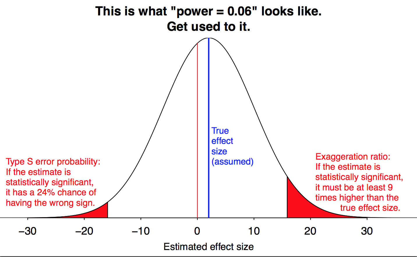
Morris’ intuition isn’t just Bayesian, as he himself notes. The final line in Morris’ table 1, which he calls “power @t”, is the (one-tailed) “severity” (sensu Deborah Mayo) of each dataset’s test of the hypothesis that the true parameter is 0.55. 1 minus the p-value is the one-tailed severity of each dataset’s test of the hypothesis that the true parameter is 0.5. All three datasets have the same p-value and so same severity against theta=0.5, but they have radically different severities against values of theta even slightly greater than 0.5. In other words, all three datasets warrant the frequentist, prior-free inference that the election is not a dead heat, and they warrant that inference to the same degree. But only the one with the largest sample size warrants the frequentist, prior-free inference that the candidate of interest is anything more than very slightly favored.
Just checked to make sure my memory wasn’t off, and yup, the frequentist intuition here concerns severity–see Deborah Mayo’s Error and the Growth of Experimental Knowledge, section 6.4, which uses the binomial distribution as a simple example.
Not that anyone else has any reason to care, but personally I’m glad that Andrew’s post today finally forced me to figure out how the notion of “severity” maps onto that wonderful “this is what power=0.06 looks like” diagram of Andrew’s. It’s been bugging me.
Jeremy:
Just came across this by chance. Maybe now you can explain the connection you find to me since I’m not seeing it and have worried about the Gelman diagram (in relation to severity): http://errorstatistics.com/2015/11/28/return-to-the-comedy-hour-p-values-vs-posterior-probabilities-1/#comment-136246
p values tell you how unlikely the data is to come from the random number generator called your null hypothesis, they don’t tell you much about what you SHOULD believe about the process.
This is an important point.
Just a clarification — p values are about the probability of extreme values under the null hypothesis. There’s still a 5% chance that I’ll draw a value with p <= 0.05. Consider drawing u from a uniform(0, 1). Then the probability that u in (0,0.025) union (0.0975,1) is the same as u being in (0.475,0.525), and they're equal width sets, but one will give you significance at p < 0.05 and one won't.
Yep, I recently blogged something kind of similar in point: http://models.street-artists.org/2015/09/03/posterior-probability-density-ratios/
We sometimes want to compare different possibilities, the ratio of the density in the vicinity of the two different possibilities is more meaningful in interpretation to a Bayesian than is the total tail probability, at least much of the time. The density ratios are dimensionless, and so don’t depend on the parameterization, which is required for them to be meaningful, and the density ratio can distinguish between the case of an unusual value even if it’s not in the tail. The tail has to decay, but there can be other portions of the space that can have low probability too (multi-modal distributions for example). If you have a mixture of two normals normal(-1,.1) and normal(1,.1) even the average is weird under the distribution!
At least I hope I’ve got it straight now; just went back and looked again and now I’m wondering if I didn’t mix something up. Clearly I should’ve had some caffeine before commenting…
Crud, having looked at this again I think my first comment is wrong and the final line in Morris’ table 1 is 1 minus the severity. Which if so would leave my intuitions very muddled. Clearly I should just stop commenting until I have my head straight.
R code:
curve(unlist(Vectorize(binom.test,vectorize.args = “p”)(x = 15, n = 20, p = x, alternative = “less”)[“p.value”,]),from = 0, to = 1, xlab = expression(theta[0]), ylab = expression(SEV(theta > theta[0])))
Adjust x and n as required.
(a), (b) and (c) would yield the same decision regardless of the type I error rate control, since they generate the same p-value. Assuming (for example) a true theta of 0.55, the corresponding type II error rates are (a) 0.888, (b) 0.593, and (c) 0.002. Given a choice between three tests with the same type I error rates but different type II error rates, any frequentist would choose the test with the lowest type II error rate, right?
But why do you assume true theta 0.55 for all cases? If you had no earthly idea what to expect for theta, the most reasonable choice would be the expected value (a) 0.75, (b) 0.575, and (c) 0.523.
I just picked 0.55 arbitrarily to illustrate the huge differences in power involved. You would see similarly huge differences of theta was 0.56, or 0.54, or whatever. The larger point is that a frequentist would want to use the test that maximizes power for a given significance level, and that points to the correct answer here.
Ram:
“Frequentist” is a mix of principles. I’m guessing that most users of classical statistical methods would see this:
A: p=.02, 95% CI (.560, .940)
C: p=.02, 95% CI (.501, .545)
and conclude that A and C are tied on the p-value criterion and that A dominates in the conf interval, so A wins, hands down. This would be a natural conclusion based on classical statistical training but in this case it would a wrong conclusion.
I agree with you that it can be very valuable to perform design calculations using prior estimates of effect sizes. In practice, though, most of the post-data design analyses I’ve seen have been based on parameter estimates from the data, in which case the experiment yielding dataset A would be analyzed conditional on the parameter value .75, and the experiment yielding dataset C would be analyzed conditional on the parameter value .523.
Andrew, if the P-values are both 0.02 then the lower bound of a 98% confidence interval is the same for both. Thus you might say that the 95% confidence intervals are a win for A, but the 98% intervals give a tie for A and B.
Michael:
Not quite because the upper bounds of the intervals are different, and the way people usually think, if you have 2 intervals with the same lower bound and different upper bounds, the one with the higher upper bound will look like the winner.
And, in any case, it’s 95% intervals that people look at.
Andrew:
Yes, I had in mind a pre-data estimate-based power analysis.
Classical statistics training, particularly of non-statisticians, may well encourage such mistakes. My point is simply that a frequentist, in deciding which test to perform, ought to care only about type I and type II error rates (provided that a binary hypothesis test is the appropriate way of formulating this research question–far from clear). Appropriate consideration of both types of error rates is sufficient to see past the mistake Morris describes, so this is really a problem of miseducation rather than a problem inherent to hypothesis testing of the frequentist sort per se.
Ram:
I don’t think it’s just miseducation. If you look at the literature on design analysis (as John Carlin and I did while working on our Perspectives on Psychological Science paper on Type S and Type M errors), you’ll see lots of warnings on why nobody should do post-data power analyses, and no papers by serious statisticians recommending post-data design calculations of any sort.
Given that Carl Morris framed his problem as post-data, I think it would be a very rare frequentist who would approach this problem as requiring a design analysis using a prior estimate of effect sizes. It’s just not something I think you’d see.
Laplace, I have wronged you.
But why a frequentist (if we think that it is someone who ignores prior information on principle) would pick up any fixed value to estimate Type II error?
Anyways, the whole point of the exercise is to show that small samples are bad beyond their tendency to generate large p-values. A true frequentist approach would be to recognize that if one works with small samples and then selects only the results with “statistically significant” p-values, it creates p-value filter and thus leads to underestimate of the true p-value. The correct analysis should go like this: these 3 measurements are a part of measuring universe with different n where only “p<0.05" trials were selected. Thus the values of p are completely irrelevant to the problem and we have to develop a statistics tailored to exactly this approach.
Two (somewhat) relevant observations:
1. In the 2004 presidential election the polls throughout October had Bush and Kerry neck and neck, with some showing a very small lead for Bush, and everyone saying it was too close to call. The final result for the popular vote came out pretty much the same – 50.7% Bush to 48.3% Kerry. (I wonder if there were there any small sample polls showing a big lead for one candidate?)
2. Those two papers in JASA 1987 were both classics in the early days of the “what’s wrong with p-values” debate. One was by Jim Berger and Thomas Sellke, the other by George Casella and Roger Berger. So if someone says that this month’s issue of the leading journal in his field has two invited papers on a certain topic with invited discussion, one by Berger and Sellke and the other by Casella and Berger, what probability would a non-statistician put on it being the same Berger?
I always think of these problems as a murder mystery.
Suppose H1 is arbitrarily close to H0 and N is small, so the null and alternative sampling distributions almost exactly overlap.
You find a significant result. Who done it? H0 or H1?
Well, given what we know about the case both are equally suspect.
I forsee my students getting very confused next year…
I think the problem is that it is counterintuitive that p(y|theta=0.5) is the same for the three experiments while, say, p(y|theta=0.45) is different. This is reflected in the stubborn idea that inconsistency with H0:theta=0.5 relates one-on-one with consistency with H1:theta>0.5.
Once you understand this counterintuitive idea, you might feel like it’s appropriate to do several hypothesis tests for different values of theta<0.5. But then how do you aggregate these tests to a single test of theta<0.5? Taking the average p-value doesn't seem right, because for example theta=0.1 is impossible so you don't want to give it any weight. You might decide to assign each p-value a weight using a measure of how close theta0 is to 0.5, giving more weight to tests of theta0 close to 0.5. And then you're almost doing Bayesian analysis with an informative prior.
+1
This seems to call for a visualization, something like this quick and dirty example of viz. the posterior probabilities.
https://dl.dropboxusercontent.com/s/luo5n817rrz8v1p/Bayes_Viz_Density.R?dl=0
But even that was not as dramatic of difference as I expected.
—-
Slightly off-topic, but are you experimenting on us with all of these clickbaity titles recently?
+1
Going a bit off-topic, I’ve been thinking in a similar computation applied to the ‘Did it replicate?’ question. It all started with this post (https://hardsci.wordpress.com/2014/07/01/some-thoughts-on-replication-and-falsifiability-is-this-a-chance-to-do-better/) by Prof. Srivastava, in which he argues that replication is a context where null-hypothesis testing might make sense. We have an estimate of the effect size, and we test a null hypothesis that the effect in the replication is equal to the previously found effect. Of course, a non-significant p-value would mean the experiment replicated.
Testing this idea with simulations (in a simple two independent samples t-test, simulating an ‘original study’ and then comparing the estimated difference between the means with a new ‘replicate study’ with the same population parameters), it seems that this procedure is biased towards rejecting the null. The p-value distribution is not uniform, but peaked at lower values. There is a 15% probability of rejecting the null at 5% significance level.
But should we really use something like the ML point estimate to test if the experiment replicate? After all, the effect size still has a lot of uncertainty associated with it. A better solution should take the estimated value and standard error to build a prior distribution (how credible is such a prior is open to discussion, given garden of forking paths, multiple comparisons and lower power problems), and compute the p-value of the replicated dataset integrating over the prior parameter values, similar to a prior predictive check. In practice, this means the final p-value is a weighted sum of various p-values, and each weight is given by the informative prior. Putting in math (I know p-values shouldn’t be treated as conditional probabilities, but the idea is already mixing everything up anyway):
P_replicate = Pr(T>t(y_replication) | theta_ml_original) (for Prof. Srivastava’s idea)
We want to take into account the uncertainy in the estimate, so:
P_replicate = Pr(T>t(y_replication)) = \int Pr(theta) * Pr(T>t(y_replication) | theta) dtheta
Testing this idea with simulations, the distribution of p-values is not uniform, too, but the proportion of p-values under 5% is, well, 5%. Or we could just do a proper prior distribution check and compare the test statistic of the replication with replicated datasets under the prior and forget about p-values.
Erikson:
I don’t think it makes sense to do a hypothesis test of the differences between the two experiments, for two reasons. First, there can always be differences; in practice there is no such thing as an identical replication, and the interesting question is what are the differences and how large (or small) are they, not a test of zero. Second, because of the garden of forking paths it can be hard to do anything at all with the published estimate from the original study.
Andrew: ” Second, because of the garden of forking paths it can be hard to do anything at all with the published estimate from the original study.”
[In the background: The crumbling sounds of the edifice of science…]
Prof. Gelman,
I understand that a hypothesis test might not be the best way to answer the ‘Did the experiment replicate?’ question. Given differences between experiments — as in the case of the replication project, with higher power and less forking — we might simply prefer the replicated experiment result as the most credible one, discarding the original, akin to what Morris suggests in his three survey results. Or we might use a more advanced technique to partially pool the estimates taking into account their differences, SE and maybe some prior information.
But, if the original experiment estimation can be trusted (maybe with a wider SE), the replication is sufficiently similar to the original, we want to give a Yes/No answer to the ‘Did it replicate’? question, and do not want to bring other prior information (is this really desirable? Not really.), the discrepancy between the replicated dataset and what we should expect under the null (the original result) seems like a good summary.
> is what are the differences and how large (or small) are they, not a test of zero.
Agree.
Here is a sketch of one way to do that – rank correlation of posterior/prior i.e. did the studies re-weight the prior probabilities similarly https://phaneron0.files.wordpress.com/2015/01/replicationplot.pdf
Keith,
Could you please explain the graph? I’m not understanding what’s going on there.
The idea seems to be: the black line moves the probability of certain values of p further away from the prior, while the red line also re-weights the belief in the same values, but to a lesser extend (given the difference in the amount of evidence in the sample, similar to Morris’s example). But what about the brown line?
I did some more testing of the ‘prior-weighted p-values’ idea and… Well, prior predictive checks (prior, in this case, taken from the original experiment) seems to be easier to compute and provide a better discrepancy summary: we can use both bayesian p-values and explore specific discrepancies.
Erikson:
OK too sketchy.
The tallest black curve is the posterior/prior (aka c * likelihood) for observing 4/20.
The shortest red curve is the posterior/prior (aka c * likelihood) for observing 2/10.
Now you can’t get more replicative than matching the observed proportions but these two are different.
Now rank the curves and they are plotted one on top of the other.
(I admittedly should have put them slightly ajar.)
So how do we deal with this huge sensitivity to the priors in Bayesian analysis? Even in this toy problem we have very little consensus over what makes a good prior do we?
And apparently the choice of prior does matter a lot in terms of the conclusions we are drawing (thanks to Bob’s code for illuminating this point).
Rahul:
What do we do with this huge sensitivity to the data model? It is what it is, we use the information we have and make assumptions as necessary.
Should we be focusing on better elicitation of consensus priors? There seems little empiricism in prior choosing.
Rahul:
In this sort of election prediction problem I think the best way to get a prior is by fitting a regression model to past data, including a variance parameter to account for variability between elections.
Andrew:
In the absence of “fitting a regression model to past data” does this have the risk of becoming a Paul Romer kind of “Mathiness”?
We can get Stan to churn out numbers accurate to three digits but the weak link in the chain is the prior choice. GIGO?
This might be a toy example but I keep seeing this at other places. A study that will go to great lengths to build an intricate model but then will just insert an ad hoc prior.
Where we can, we’ll use hierarchical models which fit the priors for a group along with the group coefficients.
History and Heuristics: In fact, there’s an approximate way of fitting a hierarchical (essentially what we’d call max marginal likelihood, as exemplified by the R package lme4) that has somewhat misleadingly been named “empirical Bayes” because it was designed with the goal of estimating priors “empirically”. The drawback to MML is that it underestimates variance in low-level parameters due to fixing the high-level parameters in the first marginal optimization step for the hierarchical parameters. An even cruder approximation is used in machine learning, where you see regularization (aka shrinkage or prior scale) tuned by cross-validation.
It’s also very important to keep in mind that a uniform prior is a choice of prior. The uniform also illustrates how priors are scale dependent (just like maximum likelihood estimation is scale dependent): uniform on log standard deviation isn’t the same as uniform on standard deviation!
One of the requirements in Bayesian analysis is to encode a “state of knowledge” into a prior distribution.
Another requirement is to describe which values of the data are credible when the model parameters take on “correct” values (usually called the likelihood but let’s be a little more general, just call it the “data model”)
Often the choice of the space in which to encode that knowledge is part of the creative task of building the model. I think it’s overlooked in many contexts especially contexts where default (linear, logistic, polynomial etc) regression models are the norm.
My impression is people neglect giving enough importance to the identification of the correct prior distribution to use.
My impression is that people neglect to really think hard about the data model !!!
Some examples:
In medicine the effectiveness of a drug treatment is in part determined by the pharmacokinetics/dynamics of the drug, the type and severity of the disease, the location of infection/inflammation/disease etc. A typical study of a new use of an existing drug might be something like post-surgically prescribing the drug in one group and a different standard drug in another group. Quite typically this is just divided into the two groups for analysis, with a single dose given, and not even the easily measured dose/mass parameter is considered, or the perfusion of the drug into the appropriate tissue (ie if surgeries are on different portions of the body…) etc etc. There are LOTS of opportunities to take into account very simple physical understanding of how conditions might alter the effectiveness of a drug… but they usually aren’t taken into account, it’s just “group A” and “group B”
In engineering: just look at the LRFD steel design handbook. It’s an enormous table of properties of different rolled-steel sections, and comes along with curves that describe the properties of a certain length of a given cross section of steel. These curves are fit via piecewise polynomials, and all the curves actually collapse down to a single formula in appropriate dimensionless form. A better single formula curve can even be derived from asymptotic matching between two regimes (the “short stubby” regime, and the “euler buckling: long/thin” regime). The data model is a hack.
In economics: witness the 3rd order polynomial with discontinuity for “distance from the river” in that study discussed here http://statmodeling.stat.columbia.edu/2013/08/05/evidence-on-the-impact-of-sustained-use-of-polynomial-regression-on-causal-inference-a-claim-that-coal-heating-is-reducing-lifespan-by-5-years-for-half-a-billion-people/ The real quantity of interest is not “distance from the river” but concentration of coal pollutant in the air. A model for that concentration could be built for each town based on simple models of weather patterns and pollution sources, and then the regression would be on the actual quantity of interest…. But, this kind of heirarchical model (where at one level you build an uncertain model for the predictor, and at another level you use the predictor to build an uncertain model for the outcome) is hard to do outside of a Bayesian analysis.
Ecology: my impression is these guys are jumping on the Bayesian causal modeling bandwagon, but for example there was an ODE fit to the Lynx/rabbit population data that blew Andrew’s mind about 5 years back.
http://statmodeling.stat.columbia.edu/2012/01/28/the-last-word-on-the-canadian-lynx-series/
etc etc etc. The big problem with many analyses is default simplistic models, and the solution is spending time to think about how the problem works, and building a model in Stan or a similar software which actually matches the physics, chemistry, social dynamics etc of the problem.
@Daniel:
These sound like bad models, yes. But is there Bayesian modelling involved here?
e.g. I was thinking of your steel handbook example because I’m most familiar with that. What’s the Bayesian angle here?
If you are talking about bad models in general then yes, I agree.
@Rahul:
Re the steel handbook. The way the LRFD design guidelines were created, they were intended to be a shorthand for a probabilistic calculation. The idea is essentially that p(Failure | load, strength) < epsilon for some epsilon. So, in a bending strength calculation, the output is supposed to be something like the epsilon quantile of strength for a dataset of beams randomly chosen from typical manufacturers.
In actual fact, as far as I understand, there was a bunch of effort made to test steel beams at universities, and develop a dataset, and various of the coefficients involved in the calculation are designed to give approximately the epsilon quantile for a specific condition. Fitting a curve through that dataset using piecewise rational functions or something was the technique used. Admittedly I think this was all begun in the 1980's so it wasn't like they could use Stan, but it WAS the case that they could use better analytical models for the strength calculation instead of just piecewise fitting through a point cloud on a scatterplot.
In my opinion, EVERY engineering problem is a Bayesian modeling problem. Some of them are problems where the delta-function approximation to the posterior is sufficient.
Suppose that the three scenarios are about people preferring a new product A (say cola) over an existing cola B in a blind taste experiment. Would you still regard c is more favorable than b and b as more favorable as a? If no, where does the difference lie?
A somewhat related question is here https://gilkalai.wordpress.com/2011/09/18/test-your-intuition-15-which-experiment-is-more-convincing/
Gil:
I’d have to think a bit more about this, but my quick intuition is Yes, C is more favorable than B, and B is more favorable than A, essentially for the reasons given by Mike in this comment. But it should be possible to come up with examples that would go the other way, for example if you had strong prior reason to believe that the new cola is much better or much worse than the existing one.
Suppose that instead of Mr Allen and Mr Baker we consider Medication A and Medication B. When we ask “what would be most encouraging to medication A” instead of “what would be most encouraging to Candidate A” the meaning of “encouraging” is different – unlike Allen and Baker we care about the margin for how much A is ahead.
Even for Allen and Baker there could be realistic scenarios for which A is more favorable than C. For example if there is a certain probability of systematic bias in the sampling. If your sampling method can lead with substantial probability to systematic bias of 2% then 15/20 might be more encouraging than 1,046/2000. For examples if 70% of the people who take the poll have tone of speech which causes 8% more Allen’s voters than Baker’s voters not to cooperate. (Such systematic biases may be even more reasonable for medications.)
Gil:
Indeed, one thing I like about statistical modeling is the way that the discussion can move from abstract questions of p-values to specific issues concerning the goals of the study or biases of measurement.
Dear Andrew, yes I agree,this is why I admire this subject. Actually (b) is in a sense most encouraging to Allen, since the reaction to (a) should be: “They sampled 20 people? we must be bankrupt” and to (c) “They sampled 2000 people, they are stealing my money”.
ICs are random intervals and, as such, they are subject to random variabilities. Their observed values alone do not signify much without their dispersion measures. It is like comparing the observed values of two estimators without regarding their standard errors or other measures. P-values can also be regarded as random variables. Identical p-values could be compared together with a measure of their variabilities. If a problem occurs in the first theory level, then you go to a meta-theory level to solve the problem, if a problem occurs in the meta-theory level, then you go to a meta-meta-theory level and so on and so forth.
It is too easy to find `apparent holes’ in the classical statistical theory, since it is a language with huge number of concepts that go far beyond the probabilistic knowledge. Unfortunately, the general recipe is: “if it appears to be probabilistically incoherent, it must be incoherent in a broadly sense and should be avoided´´. This recipe is too intellectual weak. If you do not use an appropriate language to treat these concepts that requires other non-probabilistic tools, you are doomed to interpret the classical concepts in a very narrow way as it seems the rule nowadays.
One way to interpret the classical approach is by simulating the data generating process and deriving the frequentist properties of our procedures. This is identical to Bayes. Both use generative models.
So you start with prior for theta, or an estimate from previous elections. Then:
Loop over 100,000 samples from theta
Generate population data using theta_i
Loop over 10,000 samples of size N
compute theta_estimate_ij
write theta_i and theta_estimate_ij to disk
end loop
end loop
delete all rows from the database where theta_estimate_ij is not the same to the actual estimate in the real survey.
calculate the proportion of times theta_i > 0.5.
END
That is build a generative procedure (I hesitate to call it model) to generate population data for each probable theta parameter. Apply your inferential procedure over these fake data (survey sampling). See what underlying (known) parameters are consistent with the actual estimate you observed in the real application.
Put differently, generate all possible words consistent with our beliefs, simulate runs of our inferential procedures many times over these possible worlds. Finally, condition on the actual estimate in the real application and see what possible worlds are compatible with it.
Same as Bayes but using simulation of frequentist properties instead of math.
PS I think this is what Mike’s comment at 5:39am was about. the issue is whether we are approximating Bayes (using a prior) or Bayes is approximating frequentism (simulating frequentist properties).
Fernando: You just seem to be defining Approximate Bayesian Calculation here – an extra layer would be required to calculate prior weighted confidence coverage.
So not sure what your PS was trying to get across.
Since I am random sampling from the prior the simulations should be self weighting no?
The difference is the form in which the computations are made. Consider a 1990s vintage expert system. You can either spend a lot of time populating probability tables, propagating evidence, and using probability calculus. Or, you can simply simulate data whose assimptotic frequencies mirror the probabilities.
Then inference is straightforward: Conditioning on evidence and averaging over probable (notice I did not say possible) worlds.
But to be clear. I’m shooting from the hip with a sawn-off shotgun. Just thinking out loud.
Keith: I found this simple intro to ABC https://darrenjw.wordpress.com/2013/03/31/introduction-to-approximate-bayesian-computation-abc/
Yes. What I am proposing is the same but with a minor departure. I don’t do rejection sampling. I sample without rejection. Generate multiple worlds and then condition on the evidence (i.e. subset on the rows in the simulated dataset that are consistent with the actual evidence).
The last step is as if doing rejection sampling, except it is faster over various queries.
That is, once I have the full simulated data I can condition on the evidence and remove the conditioning, and then condition on new evidence, etc.. Put differently, I can answer multiple queries with one sampling round. As opposed to having to rejection sample with each query. It simply takes more disk space but heck, nowadays they almost pay you to use disk space…
It is also more intuitive I think.
OK so you do a big simulation from a prior and save that to repeatedly condition on evidence as it comes up – re-using the sample prior multiple times.
Doing ABC when you know the likelihood is very inefficient though I believe intuitive (though I have not convinced many of this https://phaneron0.wordpress.com/2012/11/23/two-stage-quincunx-2/ ). One way to become more efficient would be to do importance sampling (re-weighting the prior to be the posterior) and sequential importance sampling (in both you could re-use a prior sample.)
Currently, if one can do it they should use Stan or other MCMC software (in seminars I used ABC and then importance sampling as training wheels for MCMC.)
Keith:
Thanks for your always helpful comments! Yesterday on the way home I was also thinking of importance sampling, etc. And sure, if you know the likelihood etc just use Stan
BUT
– Using Stan and Bayesian machinery requires a lot of prior training. Hence it remains a niche. In my view simple simulation and brute force works better for dummies like me.
– Moore’s law is on my side. My impression is that the human capacity to learning math is not getting any better. By contrast, brute force computations and data storage are getting faster and cheaper every day.
Put differently, I don’t care about efficiency. That is an engineering problem that can be solved way better than teaching people to use Bayes machinery.
At one of the Joint Statistical meetings a couple years ago, Don Rubin did say that he thought in 30 years most statistical analyses will be done with ABC – so you are in good company.
> – Using Stan and Bayesian machinery requires a lot of prior training.
That is what I think could be reduced with ABC like stuff and it was Rubin’s (1984) suggested conceptual approach for explaining Bayesian analyses – I don’t believe most need to know anything about MCMC to use Stan once they have a good sense of the challenges in sampling from the posterior and working with it.
> – Moore’s law is on my side.
The curse of dimensional is not (increasing complex analyses.
> Put differently, I don’t care about efficiency.
Not in the long run.
I have added a R demo for simple binary outcomes here https://phaneron0.wordpress.com/2012/11/23/two-stage-quincunx-2/
Keith: “The curse of dimensional is not (increasing complex analyses)”
That is true of any technology. Is the whole Peter Principle or Windows Intel thing. When you get a faster processor we don’t just stick to doing the same old things faster, and have more Margaritas in our free time.
No. We go after harder problems. So we are perennially stuck in a traffic jam.
I believe this is true of almost _any_ technology, so not a specific criticism I think.
“Identical p-values could be compared together with a measure of their variabilities.” But p-values are uniformly distributed under the null, so wouldn’t identical p-values always have identical standard errors regardless of sample size? They would be different under an alternative hypothesis, but which alternative would you chose?
Tom M,
Let “H0: theta in M0” be the null hypothesis. A p-value is defined by
p(T(x),M0) = sup_{theta in M0} P_theta(T(X) greater or equal T(x))
where t(x) is the observed value of the test statistics T(X), X=(X1,…,Xn) is the random sample and P_theta is the joint probability measure of the statistical model.
Define p(x) := p(t(x), M0), then p(X) is a random variable that depends on M0, theta and n (of course that it depends on the adopted statistical model).
You can compute, e.g., E_theta(p(X)^k) = m(k, theta). You can also estimate this variability by plugging the estimative of theta. Then, one possible measure of variability is
m(2, hat{theta}) – m(1, hat{theta})^2.
You can choose another measure if you want to.
Best.
One correction:
“p(X) is a random variable that depends on M0, theta and n (of course that it depends on the adopted statistical model)”
should be
$p(X) is a random variable whose distribution depends on M0, theta and n (of course that it depends on the adopted statistical model)”
I just happened to read a post about a similar ranking issue. The scores used to assign the ranks used a frequentist sort of technique, detailed at http://www.evanmiller.org/how-not-to-sort-by-average-rating.html
This method gives an algorithm along with the explanation that the basis of the scoring is derived from the “Lower bound of Wilson score confidence interval for a Bernoulli parameter”, from Wilson, E. B. (1927), “Probable Inference, the Law of Succession, and Statistical Inference,” Journal of the American Statistical Association, 22, 209-212.
The same author links a bayesian approach later, although it doesn’t provide such a concrete implementation… http://www.evanmiller.org/bayesian-average-ratings.html
How much does the frequentist approach described differ from the bayesian? I mean, my naive take is that the frequentist is probably ‘good enough’ and easier to implement.
Sorry, I guess after re-reading and trying an implementation, the first method really just mimics the approach of looking at confidence levels and therefore gives the poor results alluded to in this blog post.
Unfortunately for the bayesian described in the article it seems too hard to decide on an appropriate loss function. I guess that’s what all the math going back and forth in the comments is trying to address in some way. I’d like to actually recalculate the sorting in the original post in a bayesian way that led me down this rabbit hole, but I don’t think I Can follow the approach I linked.
It seems I should try to use stan actually to simulate this. But I’m intimidated since the one time I tried to set it up on windows failed horribly, and I can’t quite decide what sort of priors to use.
https://www.reddit.com/r/DotA2/comments/3ord8p/the_best_heroes_of_the_frankfurt_major_qualifiers/
Would it be appropriate to use stan and a flat prior analyze this problem? Basically, in a certain number of matches over a tournament, heroes are chosen in a picking phase… the goal is to decide which heroes were most successful based on their win rate and relative popularity. The reddit post I linked includes the data from the tournament, in the format
: (-)
Any list with an ogre mage on it is OK by me, even if it is for a card game rather than D&D proper.
The long form answer is in this paper on multiple comparisons by Gelman, Hill, and Yajima. I run an example in my Stan course and I blogged a complete example of multiple comparisons using hierarchical models way back when I was a wee Bayesian. The simple answer is use a beta prior, uniform or tighter on mean and something weakly informative on the total count (e.g., a pareto(0.1,1.5) — see chapter 5 of Gelman et al.’s Bayesian Data Analysis); but you could also use a normal prior on the logit or probit scale.
Thanks I’ve been thinking over an attempt based on this feedback, maybe will attempt tomorrow. Will update here if I ever get anything together, I appreciate the response Bob.
@hello:
I’d love to see the stan code if you ever get this done. I’m still a bit confused about how this will be coded into stan.
It’s in my definitely maybe bucket of side projects, I’ll update here if I finish it or any related implementation.
There’s a lot of problems with a ideal model for the actual hero selection / best hero selection that are glossed over in the simplistic list of “here’s 110 heroes, each was picked X times and won Y times”. I think that simple idea is the most doable and should be able to improve on the confidence interval method I linked.
The actual situation is this: In DotA hero selection, 2 teams of 5 unique heroes are selected by an alternating series of picks and “bans” (the banned heroes can’t be picked by either team). Basically both sides ban 2 heroes, pick 2, ban 2 more, pick 2 more, 1 final ban and a final pick. Specifically, for teams A & B they get the following b(an)s and p(ick)s, it’s first bans alternate, Ab#1, Bb#1, Ab#2, Bb#2, first picks given the second pick 2 in a row, Ap#1, Bp#1, Bp#2, Ap#2, and all other rounds just alternate, ie Bb#3, Ab#3, Bb#4, Ab#4, etc.
In practice, generally the perceived strongest heroes are banned in the first round of bans, because people don’t want the opposition to pick it. The first picks tend to have a couple of traits, obviously they’re perceived strong, but they also tend to be “versatile” — some heroes fit well into any lineup, while others have clear strengths and weaknesses. Teams pick the versatile heroes earlier if possible to mask their intentions — if the opposition reads your draft intentions, they can draft a lineup that counters your strategy, or ban or pick the heroes that fit in best with it.
It’s complicated in that some teams have clear strategy and player hero preferences. So a hero doing very poorly in a few games may only indicate it’s a favorite of a particularly lower skill team, the reverse can also be true, with a star team’s player skewing results. If that weren’t enough, pick preferences tend to move in some discovery cycles after the patch — some hero strategies do very well for a while, become popular until a superior strategy or specific counters are discovered decreasing its win rate.
Without getting overboard, there’s some value in a w/l sort of metric weighted on games played. I.e. this is the actually demonstrated performance. This is aimed at discovering both “hidden gems” and overrated heroes. However, ban+pick rate (or simply position in the draft when the hero is either banned or picked) is probably a better weighting system as far as popularity goes.
Intuitively, I think the first estimation should really weight the rating of the teams/players on the hero… unfortunately this is essentially a whole other can of worms since only the most successful teams tend to stay together long and its difficult for an ELO value to really settle — tracking player ELOs is ok, but team chemistry has a large impact on success.
Very interesting, all this. I’m pretty naive about rating schemes. The idea of using stan to do this intrigues me.
Pardon my non-statistican-hood. What is the Cn^2 term called? I can’t seem to find an explanation/derivation.
thanks
The Cn^2 term is the ratio of the prior variance to the posterior variance. The way to get this value is to work out the posterior distribution for \theta using the prior given at the bottom of page 131. With a little algebraic manipulation in the exponent of the normal distribution, you will end up with \exp(-(C_n*t)^2).
thanks for the tip.
I know I am getting into this really late, but I am a lost on what Morris meant by “binomial considerations” when justifying \sigma=0.5. What math-magic am I missing to make the p-value calculation work?