1. Background: Comparing a graph of data to hypothetical replications under permutation
Last year, we had a post, I’m skeptical of that claim that “Cash Aid to Poor Mothers Increases Brain Activity in Babies”, discussing recently published “estimates of the causal impact of a poverty reduction intervention on brain activity in the first year of life.”
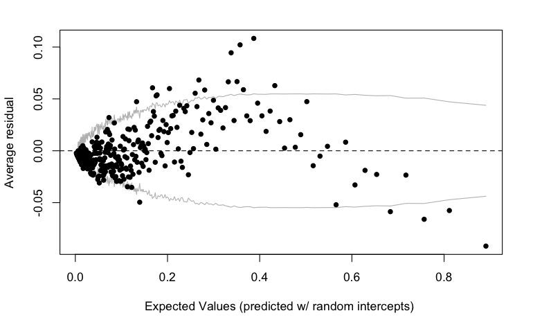
Here was the key figure in the published article:

As I wrote at the time, the preregistered plan was to look at both absolute and relative measures on alpha, gamma, and theta (beta was only included later; it was not in the preregistration). All the differences go in the right direction; on the other hand when you look at the six preregistered comparisons, the best p-value was 0.04 . . . after adjustment it becomes 0.12 . . . Anyway, my point here is not to say that there’s no finding just because there’s no statistical significance; there’s just a lot of uncertainty. The above image looks convincing but part of that is coming from the fact that the responses at neighboring frequencies are highly correlated.
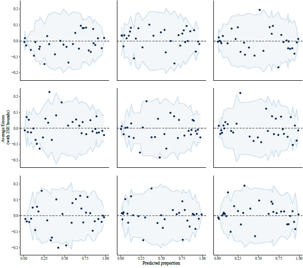
To get a sense of uncertainty and variation, I re-did the above graph, randomly permuting the treatment assignments for the 435 babies in the study. Here are 9 random instances:


2. Planning an experiment
Greg Duncan, one of the authors of the article in question, followed up:
We almost asked students in our classes to guess which of ~15 EEG patterns best conformed to our general hypothesis of negative impacts for lower frequency bands and positive impacts for higher-frequency bands. One of the graphs would be the real one and the others would be generated randomly in the same manner as in your blog post about our article. I had suggested that we wait until we could generate age and baseline-covariate-adjusted versions of those graphs . . . I am still very interested in this novel way of “testing” data fit with hypotheses — even with the unadjusted data — so if you can send some version of the ~15 graphs then I will go ahead with trying it out on students here at UCI.
I sent Duncan some R code and some graphs, and he replied that he’d try it out. But first he wrote:
Suppose we generate 14 random + 1 actual graphs; recruit, say, 200 undergraduates and graduate students; describe the hypothesis (“less low-frequency power and more high-frequency power in the treatment group relative to the control group”); and ask them to identify their top and second choices for the graphs that appear to conform most closely with the hypothesis. I would also have them write a few sentences justifying their responses in order to coax them to take the exercise seriously.
The question: how would you judge whether the responses convincingly favored the actual data? More than x% first-place votes; more than y% first or second place votes? Most votes? It would be good to pre-specify some criteria like that.
I replied that I’m not sure if the results would be definitive but I guess it would be intereseting to see what happens.
Duncan responded:
I agree that the results are merely useful but not definitive.
Your blog post used these graphs to show that the data, if manipulated with randomly-generated treatment dummies, produced an uncomfortable number of false positives. This exercise would inform that intuition, even if we want to rely on formal statistics for the most systematic assessment of how confident we should be with the results.
I agree, and Drew Bailey, who was also involved in the discussion, added:
The earlier blog post used these graphs to show that the data, if manipulated with randomly-generated treatment dummies, produced an uncomfortable number of false positives. This new exercise would inform that intuition, even if we want to rely on formal statistics for the most systematic assessment of how confident we should be with the results.
3. Experimental conditions
Duncan was then ready to go. He wrote:
I am finally ready to test randomly generated graphs out on a large classroom of undergraduate students.
Paul Yoo used Stata to generate 15 random graphs plus the real one (see attached). The position (10th) in the 16 for the PNAS graph was determined from a random number draw. (We could randomize its position but that increases the scoring task considerably.) We put an edited version of the hypothesis that was preregistered/spelled out in our original NICHD R01 proposal below the graphs. My plan is to ask class members to select their first and second choices for the graph that conforms most closely to the hypothesis.

Bailey responded:
Yes, with the same caveat as before (namely, that the paths have already forked: we aren’t looking at a plot of frequency distributions for one of the many other preregistered outcomes in part because these impacts didn’t wind up on Andrew’s blog).
4. Results
Duncan reported:
97 students examined the 16 graphs shown in the 4th slide in the attached powerpoint file. The earlier slides set up the exercise and the hypothesis.
Almost 2/3rds chose the right figure (#10) on their first guess and 78% did so on their first or second guesses. Most of the other guesses are for figures that show more treatment-group power in the beta and gamma ranges but not alpha.
5. Discussion
I’m not quite sure what to make of this. It’s interesting and I think useful to run such experiments to help stimulate our thinking.
This is all related to the 2009 paper, Statistical inference for exploratory data analysis and model diagnostics, by Andreas Buja, Dianne Cook, Heike Hofmann, Michael Lawrence, Eun-Kyung Lee, Deborah Swayne, and Hadley Wickham.
As with hypothesis tests in general, I think the value of this sort of test is when it does not reject the null hypothesis, which represents a sort of negative signal that we don’t have enough data to learn more on the topic.
The thing is, I’m not clear what to make of the result that almost 2/3rds chose the right figure (#10) on their first guess and 78% did so on their first or second guesses. On one hand, this is a lot better than the 1/16 and 1/8 we would expect by pure chance. On the other hand, the fact that some of the alternatives were similar to the real data . . . this is all getting me confused! I wonder what Buja, Cook, etc., would say about this example.
6. Expert comments
Dianne Cook responded in detail in comments. All of this is directly related to our discussion so I’m copying her comment here:
The interpretation depends on the construction of the null sets. Here you have randomised the group. There is no control of the temporal dependence or any temporal trend, so where the lines cross or the volatility of lines is possibly distracting.
You have also asked a very specific one-sided question – it took me some time to digest what your question is asking. Effectively it is, in which plot is the solid line much higher than the dashed line only in three of the zones. When you are randomising groups, the group labels have no relevance, so it would be a good idea to set the higher-valued one to be the solid line in all null sets. Otherwise, some plots would be automatically irrelevant. People don’t need to know the context of a problem to be an observer for you, and it is almost always better if the context is removed. If you had asked a different question, eg in which plot are the lines getting further apart at higher Hz, or in which plot are the two lines the most different, would likely yield different responses. The question you ask matters. We typically try to keep it generic “which plot is different” or “which plot shows the most difference between groups”. Being too specific can create the same problem as creating the hypothesis post-hoc after you have seen the data, eg you spot clusters and then do a MANOVA test. You pre-registered your hypothesis so this shouldn’t be a problem. Thus your null hypothesis is “There is NO difference in the high-frequency power between the two groups.”
When you see as much variability in the null sets as you have here, it would be recommended to make more null sets. With more variability, you need more comparisons. Unlike a conventional test where we see the full curve of the sampling distribution and can check if the observed test statistic has a value in the tails, with randomisation tests we have a finite number of draws from the sampling distribution on which to make a comparison. Numerically we could generate tons of draws but for visual testing, it’s not feasible to look at too many. However, you still might need more than your current 15 nulls to be able to gauge the extent of the variability.
For your results, it looks like 64 of the 97 students picked plot 10, their first pick. Assuming that this was done independently and that they weren’t having side conversations in the room, then you could use nullabor to calculate the p-value:
> library(nullabor)
> pvisual(64, 97, 16)
x simulated binom
[1,] 64 0 0
which means that the probability that this many people would pick plot 10, if it really was truly a null sample, is 0. Thus we would reject the null hypothesis, and with strong evidence, conclude that there is more high frequency in the high-cash group. You can include the second votes by weighting the p-value calculation by two picks out of 16 instead of one, but here the p-value is still going to be 0.
To understand whether observers are choosing the data plot, for reasons related to the hypothesis you have to ask them why they made their choice. Again, this should be very specific here because you’ve asked a very specific question, things like “the lines are constantly further apart on the right side of the plot”. For people that chose null plots instead of 10, it would be interesting to know what they were looking at. In this set of nulls, there are so many other types of differences! Plot 3 has differences everywhere. We know there are no actual group differences, so this big of an observed difference is consistent with there being no true difference. It is ruled out as a contender only because the question asks in 3 of the 4 zones if is there a difference. We see crossings of lines in many plots, so this is something very likely to see assuming the null is true. The big scissor pattern in 8 is interesting, but we know this has arisen by chance.
Well, this has taken some time to write. Congratulations on an interesting experiment, and interesting post. Care needs to be taken in designing data plots, constructing the null-generating mechanisms and wording questions appropriately when you apply the lineup protocol in practice.
This particular work has been borne from curiosity about a published data plot. It reminds me of our work in Roy Chowdhury et al (2015) (https://link.springer.com/article/10.1007/s00180-014-0534-x). It was inspired by a plot in a published paper where the authors reported clustering. Our lineup study showed that this was an incorrect conclusion, and the clustering was due to the high-dimensionality. I think your conclusion now would be that the published plot does show the high-frequency difference reported.
She also lists a bunch of relevant references at the end of the linked comment.