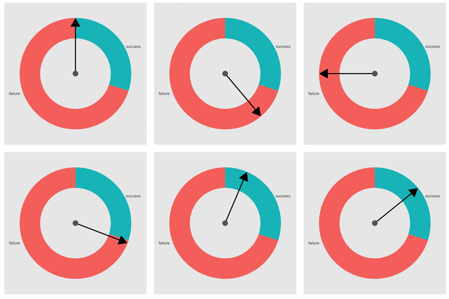
It’s Sunday, and I [Bob] am just sitting on the couch peacefully ggplotting to illustrate basic sample spaces using spinners (a trick I’m borrowing from Jim Albert’s book Curve Ball). There’s an underlying continuous outcome (i.e., where the spinner lands) and a quantization into a number of regions to produce a discrete outcome (e.g., “success” and “failure”). I’m quite pleased with myself for being able to use polar coordinates to create the spinner and arrow. ggplot works surprisingly well in polar coordinates once you figure them out; almost everything people have said about them online is confused and the doc itself assumes you’re a bit more of a ggplotter and geometer than me.
I’m so pleased with it that I show the plot to Mitzi. She replies, “Why don’t you animate it?” I don’t immediately say, “What a waste of time,” then get back to what I’m doing. Instad, I boast, “It’ll be done when you get back from your run.” Luckily for me, she goes for long runs—I just barely had the prototype working as she got home. And then I had to polish it and turn it into a blog post. So here it is, for your wonder and amazement.

Here’s the R magic.
library(ggplot2)
draw_curve <- function(angle) {
  df <- data.frame(outcome = c("success", "failure"), prob = c(0.3, 0.7))
  plot <-
    ggplot(data=df, aes(x=factor(1), y=prob, fill=outcome)) +
    geom_bar(stat="identity", position="fill") +
    coord_polar(theta="y", start = 0, direction = 1) +
    scale_y_continuous(breaks = c(0.12, 0.7), labels=c("success", "failure")) +
    geom_segment(aes(y= angle/360, yend= angle/360, x = -1, xend = 1.4), arrow=arrow(type="closed"), size=1) +
    theme(axis.title = element_blank(),
          axis.ticks = element_blank(),
          axis.text.y = element_blank()) +
    theme(panel.grid = element_blank(),
          panel.border = element_blank()) +
    theme(legend.position = "none") +
    geom_point(aes(x=-1, y = 0), color="#666666", size=5)
  return(plot)
}
ds <- c()
pos <- 0
for (i in 1:66) {
  pos <- (pos + (67 - i)) %% 360
  ds[i] <- pos
}
ds <- c(rep(0, 10), ds)
ds <- c(ds, rep(ds[length(ds)], 10))

for (i in 1:length(ds)) {
  ggsave(filename = paste("frame", ifelse(i < 10, "0", ""), i, ".png", sep=""),
         plot = draw_curve(ds[i]), device="png", width=4.5, height=4.5)
}
I probably should've combined theme functions. Ben would've been able to define ds in a one-liner and then map ggsave. I hope it's at least clear what my code does (just decrements the number of degrees moved each frame by one---no physics involved).
After producing the frames in alphabetical order (all that ifelse and paste mumbo-jumbo), I went to the output directory and ran the results through ImageMagick (which I'd previously installed on my now ancient Macbook Pro) from the terminal, using
> convert *.png -delay 3 -loop 0 spin.gif
That took a minute or two. Each of the pngs is about 100KB, but the final output is only 2.5MB or so. Maybe I should've went with less delay (I don't even know what the units are!) and fewer rotations and maybe a slower final slowing down (maybe study the physics). How do the folks at Pixar ever get anything done?
P.S. I can no longer get the animation package to work in R, though it used to work in the past. It just wraps up those calls to ImageMagick.
P.P.S. That salmon and teal color scheme is the default!