Bayes factors evaluate priors, cross validations evaluate posteriors

I’ve written this explanation on the board often enough that I thought I’d put it in a blog post.

Bayes factors

Bayes factors compare the data density (sometimes called the “evidence”) of one model against another. Suppose we have two Bayesian models for data y, one model p_1(\theta_1, y) with parameters \theta_1 and a second model p_2(\theta_2, y) with parameters \theta_2.

The Bayes factor is defined to be the ratio of the marginal probability density of the data in the two models,

\textrm{BF}_{1,2} = p_1(y) \, / \, p_2(y),

where we have

p_1(y) = \mathbb{E}[p_1(y \mid \Theta_1)] \ = \ \int p_1(y \mid \theta_1) \cdot p_1(\theta_1) \, \textrm{d}\theta_1

and

p_2(y) = \mathbb{E}[p_2(y \mid \Theta_2)] \ = \ \int p_2(y \mid \theta_2) \cdot p_2(\theta_2) \, \textrm{d}\theta_2.

The distributions p_1(y) and p_2(y) are known as prior predictive distributions because they integrate the likelihood over the prior.

There are ad-hoc guidelines from Harold Jeffreys of “uninformative” prior fame, classifying Bayes factor values as “decisive,” “very strong,” “strong,” “substantial,” “barely worth mentioning,” or “negative”; see the Wikipedia on Bayes factors. These seem about as useful as a 5% threshold on p-values before declaring significance.

Held-out validation

Held-out validation tries to evaluate prediction after model estimation (aka training). It works by dividing the data y into two pieces, y = y', y'' and then training on y' and testing on y''. The held out validation values are

p_1(y'' \mid y') = \mathbb{E}[p_1(y'' \mid \Theta_1) \mid y'] = \int p_1(y'' \mid \theta_1) \cdot p_1(\theta_1 \mid y') \, \textrm{d}\theta_1

and

p_2(y'' \mid y') = \mathbb{E}[p_2(y'' \mid \Theta_2) \mid y'] = \int p_2(y'' \mid \theta_2) \cdot p_2(\theta_2 \mid y') \, \textrm{d}\theta_2.

The distributions p_1(y'' \mid y') and p_2(y'' \mid y') are known as posterior predictive distributions because they integrate the likelihood over the posterior from earlier training data.

This can all be done on the log scale to compute either the log expected probability or the expected log probability (which are different because logarithms are not linear). We will use expected log probability in the next section.

(Leave one out) cross validation

Suppose our data is y_1, \ldots, y_N. Leave-one-out cross validation works by successively taking y'' = y_n and y' = y_1, \ldots, y_{n-1}, y_{n+1}, \ldots, y_N and then averaging on the log scale.

\frac{1}{N} \sum_{n=1}^N \log\left( \strut p_1(y_n \mid y_1, \ldots, y_{n-1}, y_{n+1}, \ldots, y_N) \right)

and

\frac{1}{N} \sum_{n=1}^N \log \left( \strut p_2(y_n \mid y_1, \ldots, y_{n-1}, y_{n+1}, \ldots, y_N) \right).

Leave-one-out cross validation is interpretable as the expected log posterior density (ELPD) for a new data item. Estimating ELPD is (part of) the motivation for various information criteria such as AIC, DIC, and WAIC.

Conclusion and a question

The main distinction between Bayes factors and cross validation is that the former uses prior predictive distributions whereas the latter uses posterior predictive distributions. This makes Bayes factors very sensitive to features of the prior that have almost no effect on the posterior. With hundreds of data points, the difference between a normal(0, 1) and normal(0, 100) prior is negligible if the true value is in the range (-3, 3), but it can have a huge effect on Bayes factors.

This matters because pragmatic Bayesians like Andrew Gelman tend to use weakly informative priors that determine the rough magnitude, but not the value of parameters. You can’t get good Bayes factors this way. The best way to get a good Bayes factor is to push the prior toward the posterior, which you get for free with cross validation.

My question is whether the users of Bayes factors really believe so strongly in their priors. I’ve been told that’s true of the hardcore “subjective” Bayesians, who aim for strong priors, and also the hardcore “objective” Bayesians, who try to use “uninformative” priors, but I don’t think I’ve ever met anyone who claimed to follow either approach. It’s definitely not the perspective we’ve been pushing in our “pragmatic” Bayesian approach, for instance as described in the Bayesian workflow paper. We flat out encourage people to start with weakly informative priors and then add more information if the priors turn out to be too weak for either inference or computation.

Further reading

For more detail on these methods and further examples, see Gelman et al.’s Bayesian Data Analysis, 3rd Edition, which is available free online through the link, particularly Section 7.2 (“Information criteria and cross-validation,” p. 175) and section 7.4 (“Model comparison using Bayes factors,” page 183). I’d also recommend Vehtari, Gelman, and Gabry’s paper, Practical Bayesian model evaluation using leave-one-out cross-validation and WAIC.

Difference-in-differences: What’s the difference?

After giving my talk last month, Better Than Difference in Differences, I had some thoughts about how diff-in-diff works—how the method operates in relation to its assumptions—and it struck me that there are two relevant ways to think about it.

From a methods standpoint the relevance here is that I will usually want to replace differencing with regression. Instead of taking (yT – yC) – (xT – xC), where T = Treatment and C = Control, I’d rather look at (yT – yC) – b*(xT – xC), where b is a coefficient estimated from the data, likely to be somewhere between 0 and 1. Difference-in-differences is the special case b=1, and in general you should be able to do better by estimating b. We discuss this with the Electric Company example in chapter 19 of Regression and Other Stories and with a medical trial in our paper in the American Heart Journal.

Given this, what’s the appeal of diff-in-diff? I think the appeal of the method comes from the following mathematical sequence:

Control units:
(a) Data at time 0 = Baseline + Error_a
(b) Data at time 1 = Baseline + Trend + Error_b

Treated units:
(c) Data at time 0 = Baseline + Error_c
(d) Data at time 1 = Baseline + Trend + Effect + Error_d

Now take a diff in diff:

((d) – (c)) – ((b) – (a)) = Effect + Error,

where that last Error is a difference in difference of errors, which is just fine under the reasonable-enough assumption that the four error terms are independent.

The above argument looks pretty compelling and can easily be elaborated to include nonlinear trends, multiple time points, interactions, and so forth. That’s the direction of the usual diff-in-diff discussions.

The message of my above-linked talk and our paper, though, was different. Our point was that, whatever differencing you take, it’s typically better to difference only some of the way. Or, to make the point more generally, it’s better to model the baseline and the trend as well as the effect.

Seductive equations

The above equations are seductive: with just some simple subtraction, you can cancel out Baseline and Trend, leaving just Effect and error. And the math is correct (conditional on the assumptions, which can be reasonable). The problem is that the resulting estimate can be super noisy; indeed, it’s basically never the right thing to do from a probabilistic (Bayesian) standpoint.

In our example it was pretty easy in retrospect to do the fully Bayesian analysis. It helped that we had 38 replications of similar experiments, so we could straightforwardly estimate all the hyperparameters in the model. If you only have one experiment, your inferences will depend on priors that can’t directly be estimated from local data. Still, I think the Bayesian approach is the way to go, in the sense of yielding effect-size estimates that are more reasonable and closer to the truth.

Next step is to work this out on some classic diff-in-diff examples.

Donald Trump’s and Joe Biden’s ages and conditional probabilities of their dementia risk

The prior

Paul Campos posted something on the ages of the expected major-party candidates for next year’s presidential election:

Joe Biden is old. Donald Trump is also old. A legitimate concern about old people in important positions is that they are or may become cognitively impaired (For example, the prevalence of dementia doubles every five years from age 65 onward, which means that on average an 80-year-old is is eight times more likely to have dementia than a 65 year old).

Those are the baseline probabilities, which is one reason that Nate Silver wrote:

Of course Biden’s age is a legitimate voter concern. So is Trump’s, but an extra four years makes a difference . . . The 3.6-year age difference between Biden and Trump is potentially meaningful, at least based on broad population-level statistics. . . . The late 70s and early 80s are a period when medical problems often get much worse for the typical American man.

Silver also addressed public opinion:

An AP-NORC poll published last week found that 77 percent of American adults think President Biden is “too old to be effective for four more years”; 51 percent of respondents said the same of Donald Trump. . . . the differences can’t entirely be chalked up to partisanship — 74 percent of independents also said that Biden was too old, while just 48 percent said that of Trump.

The likelihood

OK, those are the base rates. What about the specifics of this case? Nate compares to other politicians but doesn’t offer anything about Biden or Trump specifically.

Campos writes:

Recently, Trump has been saying things that suggest he’s becoming deeply confused about some very basic and simple facts. For example, this weekend he gave a speech in which he seemed to be under the impression that Jeb Bush had as president launched the second Iraq war . . . In a speech on Friday, Trump claimed he defeated Barack Obama in the 2016 presidential election. . . . Trump also has a family history of dementia, which is a significant risk factor in terms of developing it himself.

Campos notes that Biden’s made his own slip-ups (“for example he claimed recently that he was at the 9/11 Twin Towers site the day after the attack, when in fact it was nine days later”) and summarizes:

I think it’s silly to deny that Biden’s age isn’t a legitimate concern in the abstract. Yet based on the currently available evidence, Trump’s age is, given his recent ramblings, a bigger concern.

It’s hard to know. A quick google turned up this:

On July 21, 2021, during a CNN town hall, President Joe Biden was asked when children under 12 would be able to get COVID-19 vaccinations. Here’s the start of his answer to anchor Don Lemon: “That’s under way just like the other question that’s illogical, and I’ve heard you speak about it because y’all, I’m not being solicitous, but you’re always straight up about what you’re doing. And the question is whether or not we should be in a position where you uh um, are why can’t the, the, the experts say we know that this virus is in fact uh um uh is, is going to be, excuse me.”

On June 18, after Biden repeatedly confused Libya and Syria in a news conference, The Washington Post ran a long story about 14 GOP lawmakers who asked Biden to take a cognitive test. The story did not note any of the examples of Biden’s incoherence and focused on, yes, Democrats’ concerns about Trump’s mental health.

And then there’s this, from a different news article:

Biden has also had to deal with some misinformation, including the false claim that he fell asleep during a memorial for the Maui wildfire victims. Conservatives — including Fox News host Sean Hannity — circulated a low-quality video on social media to push the claim, even though a clearer version of the moment showed that the president simply looked down for about 10 seconds.

There’s a lot out there on the internet. One of the difficulties with thinking about Trump’s cognitive capacities is that he’s been saying crazy things for years, so when he responds to a question about the Russia-Ukraine war by talking about windmills, that’s compared not to a normal politician but with various false and irrelevant things he’s been saying for years.

I’m not going to try to assess or summarize the evidence regarding Biden’s or Trump’s cognitive abilities—it’s just too difficult given that all we have is anecdotal evidence. Both often seem disconnected from the moment, compared to previous presidents. And, yes, continually being in the public eye can expose weaknesses. And Trump’s statements have been disconnected from reality for so long, that this seems separate from dementia even if it could have similar effects from a policy perspective.

Combining the prior and the likelihood

When comparing Biden and Trump regarding cognitive decline, we have three pieces of information:

1. Age. This is what I’m calling the base rate, or prior. Based on the numbers above, someone of Biden’s age is about 1.6 times more likely to get dementia than someone of Trump’s age.

2. Medical and family history. This seems less clear, but from the above information it seems that someone with Trump’s history is more at risk of dementia than someone with Biden’s.

3. Direct observation. Just so hard to compare. That’s why there are expert evaluations, but it’s not like a bunch of experts are gonna be given access to evaluate the president and his challenger.

This seems like a case where data source 3 should have much more evidence than 1 and 2. (It’s hard for me to evaluate 1 vs. 2; my quick guess would be that they are roughly equally relevant.) But it’s hard to know what to do with 3, given that no systematic data have been collected.

This raises an interesting statistical point, which is how to combine the different sources of information. Nate Silver looks at item 1 and pretty much sets aside items 2 and 3. In contrast, Paul Campos says that 1 and 2 pretty much cancel and that the evidence from item 3 is strong.

I’m not sure what’s the right way to look at this problem. I respect Silver’s decision not to touch item 3 (“As of what to make of Biden and Trump in particular — look, I have my judgments and you have yours. Cognitively, they both seem considerably less sharp to me than they did in their primes”); on the other hand, there seems to be so much direct evidence, that I’d think it would overwhelm a base rate odds of 1.6.

News media reporting

The other issue is news media coverage. Silver argues that the news media should be spending more time discussing the statistical probability of dementia or death as a function of age, in the context of Biden and Trump, and one of his arguments is that voters are correct to be more concerned about the health of the older man.

Campos offers a different take:

Nevertheless, Biden’s age is harped on ceaselessly by the media, while Trump apparently needs to pull a lampshade over his head and start talking about how people used to wear onions on their belts before the same media will even begin to talk about the exact same issue in regard to him, and one that, given his recent behavior, seems much more salient as a practical matter.

From Campos’s perspective, voters’ impressions are a product of news media coverage.

But on the internet you can always find another take, such as this from Roll Call magazine, which quotes a retired Democratic political consultant as saying, “the mainstream media has performed a skillful dance around the issue of President Biden’s age. . . . So far, it is kid gloves coverage for President Biden.” On the other hand, the article also says, “Then there’s Trump, who this week continued his eyebrow-raising diatribes on his social media platform after recently appearing unable, at times, to communicate complete thoughts during a Fox News interview.”

News coverage in 2020

I recall that age was discussed a lot in the news media during the 2020 primaries, where Biden and Sanders were running against several much younger opponents. It didn’t come up so much in the 2020 general election because (a) Trump is almost as old as Biden, and (b) Trump had acted so erratically as president that it was hard to line up his actual statements and behaviors with a more theoretical, actuarial-based risk based on Biden’s age.

Statistical summary

Comparing Biden and Trump, it’s not clear what to do with the masses of anecdotal data; on the other hand, it doesn’t seem quite right to toss all that out and just go with the relatively weak information from the base rates.

I guess this happens a lot in decision problems. You have some highly relevant information that is hard to quantify, along with some weaker, but quantifiable statistics. In their work on cognitive illusions, Tversky and Kahneman noted the fallacy of people ignoring base rates, but there can be the opposite problem of holding on to base rates too tightly, what we’ve called slowness to update. In general, we seem to have difficulty balancing multiple pieces of information.

P.S. Some discussion in comments about links between age and dementia, or diminished mental capacities, also some discussion about evidence for Trump’s and Biden’s problems. The challenge remains of how to put these two pieces of information together. I find it very difficult to think about this sort of question where the available data are clearly relevant yet have such huge problems with selection. There’s a temptation to fall back on base rates but that doesn’t seem right to me either.

P.P.S. I emailed Campos and Silver regarding this post. Campos followed up here. I didn’t hear back from Silver, but I might not have his current email, so if anyone has that, could you please send it to me? Thanks.

My SciML Webinar next week (28 Sep): Multiscale generalized Hamiltonian Monte Carlo with delayed rejection

I’m on the hook to do a SciML webinar next week:

These are organized by Keith Phuthi (who is at CMU) through University of Michigan’s Institute for Computational Discovery and Engineering.

Sam Livingstone is moderating.This is presenting joint work with Alex Barnett, Chirag Modi, Edward Roualdes, and Gilad Turok.

I’m very excited about this project as it combines a number of threads I’ve been working on with collaborators. When I did my job talk here, Leslie Greengard, our center director, asked me why we didn’t use variable stepwise integrators when doing Hamiltonian Monte Carlo. I told him we’d love to do it, but didn’t know how to do it in such a way as to preserve the stationary target distribution.

Delayed rejection HMC

Then we found Antonietta Mira’s work on delayed rejection. It lets you retry a second Metropolis proposal if the first one is rejected. The key here is that we can use a smaller step size for the second proposal, thus recovering from proposals that are rejected because the Hamiltonian diverged (i.e., the first-order gradient based algorithm can’t handle regions of high curvature in the target density). There’s a bit of bookkeeping (which is frustratingly hard to write down) for the Hastings condition to ensure detailed balance. Chirag Modi, Alex Barnett and I worked out the details, and Chirag figured out a novel twist on delayed rejection that only retries if the original acceptance probability was low. You can read about it in our paper:

This works really well and is enough that we can get proper draws from Neal’s funnel (vanilla HMC fails on this example in either the tails in either the mouth or neck of the funnel, depending on the step size). But it’s inefficient in that it retries an entire Hamiltonian trajectory. Which means if we cut the step size in half, we double the number of steps to keep the integration time constant.

Radford Neal to the rescue

As we were doing this, the irrepressible Radford Neal published a breakthrough algorithm:

What he managed to do was use generalized Hamiltonian Monte Carlo (G-HMC) to build an algorithm that takes one step of HMC (like Metropolis-adjusted Langevin, but over the coupled position/momentum variables) and manages to maintain directed progress. Instead of fully resampling momentum each iteration, G-HMC resamples a new momentum value then performs a weighted average with the existing momentum with most of the weight on the existing momentum. Neal shows that with a series of accepted one-step HMC iterations, we can make directed progress just like HMC with longer trajectories. The trick is getting sequences of acceptances together. Usually this doesn’t work because we have to flip momentum each iteration. We can re-flip it when regenerating, to keep going in the same direction on acceptances, but with rejections we reverse momentum (this isn’t an issue with HMC because it fully regenerates each time). So to get directed movement, we need steps that are too small. What Radford figured out is that we can solve this problem by replacing the way we generate uniform(0, 1)-distributed probabilities for the Metropolis accept/reject step (we compare the variate generated to the ratio of the density at the proposal to the density at the previous point and accept if it’s lower). Radford realized that if we instead generate them in a sawtooth pattern (with micro-jitter for ergodicity), then when we’re at the bottom of the sawtooth generating a sequence of values near zero, the acceptances will cluster together.

Replacing Neal’s trick with delayed rejection

Enter Chirag’s and my intern, Gilad Turok (who came to us as an undergrad in applied math at Columbia). Over the summer, working with me and Chirag and Edward Roualdes (who was here as a visitor), he built and evaluated a system that replaces Neal’s trick (sawtooth pattern of acceptance probability) with the Mira’s trick (delayed rejection). It indeed solves the multi scale problem. It exceeded our expectations in terms of efficiency—it’s about twice as fast as our delayed rejection HMC. Going one HMC step at a time, it is able to adjust its stepsize within what would be a single Hamiltonian trajectory. That is, we finally have something that works roughly like a typical ODE integrator in applied math.

Matt Hoffman to the rescue

But wait, that’s not all. There’s room for another one of the great MCMC researchers to weigh in. Matt Hoffman, along with Pavel Sountsov, figured out how to take Radford’s algorithm and provide automatic adaptation for it.

What Hoffman and Sountsov manage to do is run a whole lot of parallel chains, then use information in the other chains to set tuning parameters for a given chain. In that way it’s like the Goodman and Weare affine-invariant sampler that’s used in the Python package emcee. This involves estimating the metric (posterior covariance or just variance in the diagonal case) and also estimating steps size, which they do through a heuristic largest-eigenvalue estimate. Among the pleasant properties of their approach is that the entire setup produces a Markov chain from the very first iteration. That means we only have to do what people call “burn in” (sorry Andrew, but notice how I say other people call it that, not that they should), not set aside some number of iterations for adaptation.

Edward Roualdes has coded up Hoffman and Sountsov’s adaptation and it appears to work with delayed rejection replacing Neal’s trick.

Next for Stan?

I’m pretty optimistic that this will wind up being more efficient than NUTS and also make things like parallel adaptation and automatic stopping a whole lot easier. It should be more efficient because it doesn’t waste work—NUTS goes forward and backward in time and then subsamples along the final doubling (usually—it’s stochastic with a strong bias toward doing that). This means we “waste” the work going the wrong way in time and beyond where we finally sample. But we still have a lot of eval to do before we can replace Stan’s longstanding sampler or even provide an alternative.

My talk

The plan’s basically to expand this blog post with details and show you some results. Hope to see you there!

How big problem it is that cross-validation is biased?

Some weeks ago, I posted in Mastodon (you can follow me there) a thread about “How big problem it is that cross-validation is biased?”. I have also added that text to CV-FAQ. Today I extended that thread as we have a new paper out on estimating and correcting selection induced bias in cross-validation model selection.

I’m posting here the whole thread for the convenience of those who are not (yet?) following me in Mastodon:

Unbiasedness has a special role in statistics, and too often there are dichotomous comments that something is not valid or is inferior because it’s not unbiased. However, often the non-zero bias is negligible, and often by modifying the estimator we may even increase bias but reduce the variance a lot, providing an overall improved performance.

In CV the goal is to estimate the predictive performance for unobserved data given the observed data of size n. CV has pessimistic bias due to using less than n observation to fit the models. In case of LOO-CV this bias is usually small and negligible. In case of K -fold-CV with a small K, the bias can be non-negligible, but if the effective number of parameters of the model is much less than n, then with K>10 the bias is also usually negligible compared to the variance.

There is a bias correction approach by Burman (1989) (see also Fushiki (2011)) that reduces CV bias, but even in the cases with non-negligible bias reduction, the variance tends to increase so much that there is no real benefit (see, e.g. Vehtari and Lampinen (2002)).

For time series when the task is to predict future (there are other possibilities like missing data imputation) there are specific CV methods such as leave-future-out (LFO) that have lower bias than LOO-CV or K -fold-CV (Bürkner, Gabry and Vehtari, 2020). There are sometimes comments that LOO-CV and K -fold-CV would be invalid for time series. Although they tend to have a bigger bias than LFO, they are still valid and can be useful, especially in model comparison where bias can cancel out.

Cooper et al. (2023) demonstrate how in time series model comparison variance is likely to dominate, it is more important to reduce the variance than bias, and leave-few-observations and use of joint log score is better than use of LFO. The problem with LFO is that the data sets used for fitting models are smaller, increasing the variance.

Bengio and Grandvalet (2004) proved that there is no unbiased estimate for the variance of CV in general, which has been later used as an argument that there is no hope. Instead of dichotomizing to unbiased or biased, Sivula, Magnusson and Vehtari (2020) consider whether the variance estimates are useful and how to diagnose when the bias is likely to not be negligible (Sivula, Magnusson and Vehtari (2023) prove also a special case where there actually exists unbiased variance estimate).

CV tends to have high variance, as the sample reuse is not making any modeling assumptions (this holds also for information criteria such as WAIC). Not making modeling assumptions is good when we don’t trust our models, but if we trust we can get reduced variance in model comparison, for example, examining directly the posterior or using reference models to filter out noise in the data (see, e.g., Piironen, Paasiniemi and Vehtari (2018) and Pavone et al. (2020)).

When using CV (or information criteria such as WAIC) for model selection, the performance estimate for the selected model has additional selection induced bias. In case of small number of models this bias is usually negligible, that is, smaller than the standard deviation of the estimate or smaller than what is practically relevant. In case of negligible bias, we may choose suboptimal model, but the difference to the performance of oracle model is small.

In case of a large number of models the selection induced bias can be non-negligible, but this bias can be estimated using, for example, nested-CV or bootstrap. The concept of the selection induced bias and related potentially harmful overfitting are not new concepts, but there hasn’t been enough discussion when they are negligible or non-negligible.

In our new paper with Yann McLatchie Efficient estimation and correction of selection-induced bias with order statistics we review the concepts of selection-induced bias and overfitting, propose a fast to compute estimate for the bias, and demonstrate how this can be used to avoid selection induced overfitting even when selecting among 10^30 models.

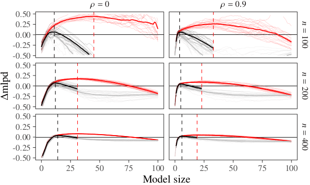
The figure here shows simulation results with p=100 covariates, with different data sizes n, and varying block correlation among the covariates. The red lines show the LOO-CV estimate for the best model chosen so far in forward-search. The grey lines show the independent, much bigger test data performance, which usually don’t have available. The black line shows our corrected estimate taking into account the selection induced bias. Stopping the searches at the peak of black curves avoids overfitting.
The figure here shows simulation results with p=100 covariates, with different data sizes n, and varying block correlation among the covariates. The red lines show the LOO-CV estimate for the best model chosen so far in forward-search. The grey lines show the independent much bigger test data performance, which usually don't have available. Black line shows our corrected estimate taking into account the selection induced bias. Stopping the searches at the peak of black curves avoids overfitting.

Although we can estimate and correct the selection induced bias, we primarily recommend to use more sensible priors and not to do model selection. See more in Efficient estimation and correction of selection-induced bias with order statistics and Bayesian Workflow.

Using forecasts to estimate individual variances

Someone who would like to remain anonymous writes:

I’m a student during the school year, but am working in industry this summer. I am currently attempting to overhaul my company’s model of retail demand. We advise suppliers to national retailers, our customers are suppliers. Right now, for each of our customers, our demand model outputs a point estimate of how much of their product will be consumed at one of roughly a hundred locations. This allows our customers to decide how much to send to each location.

However, because we are issuing point estimates of mean demand, we are *not* modeling risk directly, and I want to change that, as understanding risk is critical to making good decisions about inventory management – the entire point of excess inventory is to provide a buffer against surprises.

Additionally, the model currently operates on a per-day basis, so that predictions for a month from now are obtained by chaining together thirty predictions about what day N+1 will look like. I want to change that too, because it seems to be causing a lot of problems with errors in the model propagating across time, to the point that predictions over even moderate time intervals are not reliable.

I already know how to do both of these in an abstract way.

I’m willing to bite the bullet of assuming that the underlying distribution of the PDF should be multivariate Gaussian. From there, arriving at the parameters of that PDF just requires max likelihood estimation. For the other change, without going into a lot of tedious detail, Neural ODE models are flexible with respect to time such that you can use the same model to predict the net demand accumulated over t=10 days as you would to predict the net demand accumulated over t=90 days, just by changing the time parameter that you query the model with.

The problem is, although I know how to build a model that will do this, I want the estimated variance for each customer’s product to be individualized. Yet frustratingly, in a one-shot scenario, the maximum likelihood estimator of variance is zero. The only datapoint I’ll have to use to train the model to estimate the mean aggregate demand for, say, cowboy hats in Seattle at time t=T (hereafter (c,S,T)) is the actual demand for that instance, so the difference between the mean outcome and the actual outcome will be zero.

It’s clear to me that if I want to arrive at a good target for variance or covariance in order to conduct risk assessment, I need to do some kind of aggregation over the outcomes, but most of the obvious options don’t seem appealing.

– If I obtain an estimate of variance by thinking about the difference between (c,S,T) and (c,Country,T), aggregating over space, I’m assuming that each location shares the same mean demand, which I know is false.

– If I obtain one by thinking about the difference between (c,S,T) and (c,S,tbar), aggregating over time, I am assuming there’s a stationary covariance matrix for how demand accumulates at that location over time, which I know is false. This will fail especially badly if issuing predictions across major seasonal events, such as holidays or large temperature changes.

– If I aggregate across customers by thinking about the difference between (c,S,T) and (cbar,S,T), I’ll be assuming that the demand for cowboy hats at S,T should obey similar patterns as the demand for other products, such as ice cream or underwear sales, which seems obviously false.

I have thought of an alternative to these, but I don’t know if it’s even remotely sensible, because I’ve never seen anything like it done before. I would love your thoughts and criticisms on the possible approach. Alternatively, if I need to bite the bullet and go with one of the above aggregation strategies instead, it would benefit me a lot to have someone authoritative tell me so, so that I stop messing around with bad ideas.

My thought was that instead of asking the model to use the single input vector associated with t=0 to predict a single output vector at t=T, I could instead ask the model to make one prediction per input vector for many different input vectors from the neighborhood of time around t=0 in order to predict outcomes at a neighborhood of time around t=T. For example, I’d want one prediction for t=-5 to t=T, another prediction for t=-3 to t=T+4, and so on.

I would then judge the “true” target variance for the model relative to the difference between (c,S,T)’s predicted demand and the average of the model’s predicted demands for those nearby time slices. The hope is that this would reasonably correspond to the risks that customers should consider when optimizing their inventory management, by describing the sensitivity of the model to small changes in the input features and target dates it’s queried on. The model’s estimate of its own uncertainty wouldn’t do a good job of representing out-of-model error, of course, but the hope is that it’d at least give customers *something*.

Does this make any sense at all as a possible approach, or am I fooling myself?

My reply: I haven’t followed all the details, but my guess is that your general approach is sound. It should be possible to just fit a big Bayesian model in Stan, but maybe that would be too slow, I don’t really know how big the problem is. The sort of approach described above, where different models are fit and compared, can be thought of as a kind of computational approximation to a more structured hierarchical model, in the same way that cross-validation can be thought of as an approximation to an error model, or smoothing can be thought of as an approximation to a time-series model.

Improving Survey Inference in Two-phase Designs Using Bayesian Machine Learning

Xinru Wang, Lauren Kennedy, and Qixuan Chen write:

The two-phase sampling design is a cost-effective sampling strategy that has been widely used in public health research. The conventional approach in this design is to create subsample specific weights that adjust for probability of selection and response in the second phase. However, these weights can be highly variable which in turn results in unstable weighted analyses. Alternatively, we can use the rich data collected in the first phase of the study to improve the survey inference of the second phase sample. In this paper, we use a Bayesian tree-based multiple imputation (MI) approach for estimating population means using a two-phase survey design. We demonstrate how to incorporate complex survey design features, such as strata, clusters, and weights, into the imputation procedure. We use a simulation study to evaluate the performance of the tree-based MI approach in comparison to the alternative weighted analyses using the subsample weights. We find the tree-based MI method outperforms weighting methods with smaller bias, reduced root mean squared error, and narrower 95% confidence intervals that have closer to the nominal level coverage rate. We illustrate the application of the proposed method by estimating the prevalence of diabetes among the United States non-institutionalized adult population using the fasting blood glucose data collected only on a subsample of participants in the 2017-2018 National Health and Nutrition Examination Survey.

Yes, weights can be variable! Poststratification is better, but we don’t always have the relevant information. Imputation is a way to bridge the gap. Imputations themselves are model-dependent and need to be checked. Still, the alternatives of ignoring design calculations or relying on weights have such problems of their own, that I think that modeling is the way to go. Further challenges will arise such as imputing cluster membership in the population.

When I said, “judge this post on its merits, not based on my qualifications,” was this anti-Bayesian? Also a story about lost urine.

Paul Alper writes, regarding my post criticizing an epidemiologist and a psychologist who were coming down from the ivory tower to lecture us on “concrete values like freedom and equality”:

In your P.P.S. you write,

Yes, I too am coming down from the ivory tower to lecture here. You’ll have to judge this post on its merits, not based on my qualifications. And if I go around using meaningless phrases such as “concrete values like freedom and equality,” please call me on it!

While this sounds reasonable, is it not sort of anti-Bayes? By that I mean your qualifications represent a prior and the merits the (new) evidence. I am not one to revere authority but deep down in my heart, I tend to pay more attention to a medical doctor at the Mayo Clinic than I do to Stella Immanuel. On the other hand, decades ago the Mayo Clinic misplaced (lost!) a half liter of my urine and double charged my insurance when getting a duplicate a few weeks later.

Alper continues:

Upon reflection—this was over 25 years ago—a half liter of urine does sound like an exaggeration, but not by much. The incident really did happen and Mayo tried to charge for it twice. I certainly have quoted it often enough so it must be true.

On the wider issue of qualifications and merit, surely people with authority (degrees from Harvard and Yale, employment at the Hoover Institution, Nobel Prizes) are given slack when outlandish statements are made. James Watson, however, is castigated exceptionally precisely because of his exceptional longevity.

I don’t have anything to say about the urine, but regarding the Bayesian point . . . be careful! I’m not saying to make inferences or make decisions solely based on local data, ignoring prior information coming from external data such as qualifications. What I’m saying is to judge this post on its merits. Then you can make inferences and decisions in some approximately Bayesian way, combining your judgment of this post with your priors based on your respect for my qualifications, my previous writings, etc.

This is related to the point that a Bayesian wants everybody else to be non-Bayesian. Judge my post on its merits, then combine with prior information. Don’t double-count the prior.

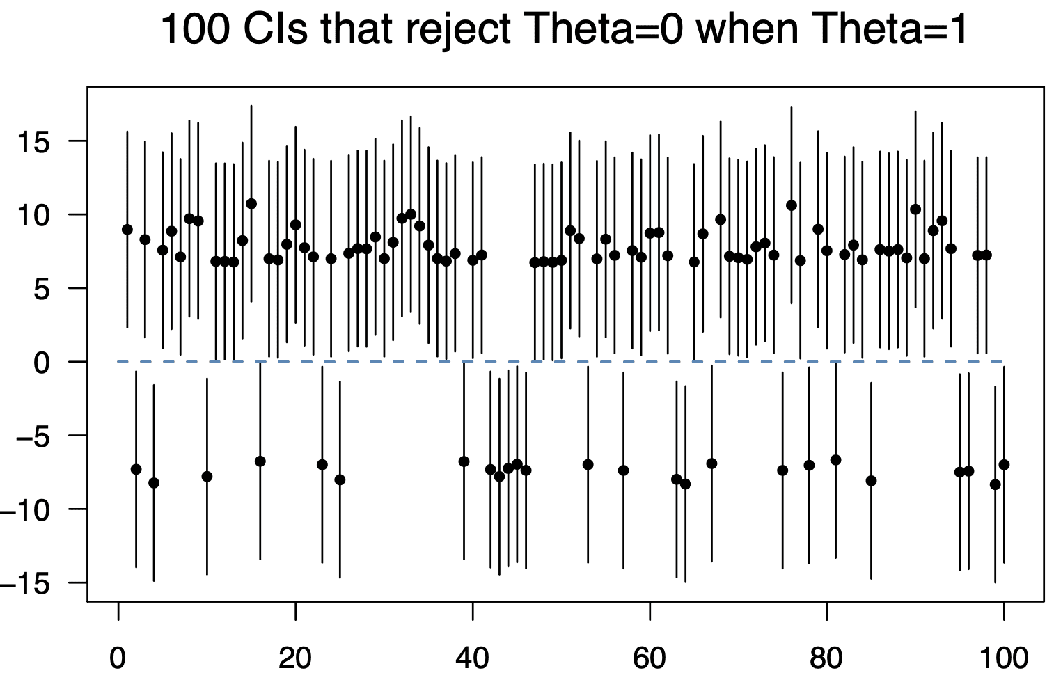
This is what “power = .06” looks like (visualized by Art Owen).

Art Owen writes:

Here’s a figure you might like. I generated a bunch of data sets constructed to have true effect size 1 and power equal to 0.06. The first 100 confidence intervals that exclude 0 are shown. Their endpoints come close to the origin and their centers have absolute value far from 1. Just over 1/4 of them have the wrong sign.

When the CI endpoint is a full CI width away from zero, then you’d be pretty safe regarding the sign. Details are in this article.

I do like the above figure. It’s a very vivid expression of This is what “power = .06” looks like. Get used to it. Somebody should send it to the University of Chicago economics department.

PhD student, PostDoc, and Research software engineering positions

Several job opportunities in beautiful Finland!

  1. Fully funded postdoc and doctoral student positions in various topics including Bayesian modeling, probabilistic programming and workflows with me and other professors in Aalto University and University of Helsinki, funded by Finnish Center for Artificial Intelligence

    See more topics, how to apply, and job details like salary at fcai.fi/we-are-hiring

    You can also ask me for further details

  2. Permanent full time research software engineer position at Aalto University. Aalto Scientific Computing is a specialized type of research support, providing high-performance computing hardware, management, research support, teaching, and training. The team works with top researchers throughout the university. All the work is open-source by default and the team take an active part in worldwide projects.

    See more about tasks, qualifications, salary, etc in www.aalto.fi/en/open-positions/research-software-engineer

    This could be a great fit also for someone interested in probabilistic programming. I know some of the RSE group members, and they are great, and we’ve been very happy to get their help, e.g. in developing priorsense package.

There are no underpowered datasets; there are only underpowered analyses.

Is it ok to pursue underpowered studies?

This question comes from Harlan Campbell, who writes:

Recently we saw two different about commentaries on the importance of pursuing underpowered studies, both with arguments motivated by thoughts on COVID-19 research:

COVID-19: underpowered randomised trials, or no randomised trials? by Atle Fretheim

and
Causal analyses of existing databases: no power calculations required by Miguel Hernán

Both explain the important idea that underpowered/imprecise studies “should be viewed as contributions to the larger body of evidence” and emphasize that several of these studies can, when combined together in a meta-analysis, “provide a more precise pooled effect estimate”.

Both sparked quick replies:
https://doi.org/10.1186/s13063-021-05755-y
https://doi.org/10.1016/j.jclinepi.2021.09.026
https://doi.org/10.1016/j.jclinepi.2021.09.024
and lastly from myself and others:
https://doi.org/10.1016/j.jclinepi.2021.11.038

and even got some press.

My personal opinion is that there are both costs (e.g., wasting valuable resources, furthering distrust in science) and benefits (e.g., learning about an important causal question) to pursuing underpowered studies. The trade-off may indeed tilt towards the benefits if the analysis question is sufficiently important; much like driving through a red light on-route to the hospital might be advisable in a medical emergency, but should otherwise be avoided. In the latter situation, risks can be mitigated with a trained ambulance driver at the wheel and a wailing siren. When it comes to pursuing underpowered studies, there are also ways to minimize risks. For example, by committing to publish one’s results regardless of the outcome, by pre-specifying all of one’s analyses, and by making the data publicly available, one can minimize the study’s potential contribution to furthering distrust in science. That’s my two cents. In any case, it certainly is an interesting question.

I agree with the general principle that data are data, and there’s nothing wrong with gathering a little bit of data and publishing what you have, in the hope that it can be combined now or later with other data and used to influence policy in an evidence-based way.

To put it another way, the problem is not “underpowered studies”; it’s “underpowered analyses.”

In particular, if your data are noisy relative to the size of the effects you can reasonably expect to find, then it’s a big mistake to use any sort of certainty thresholding (whether that be p-values, confidence intervals, posterior intervals, Bayes factors, or whatever) in your summary and reporting. That would be a disaster—type M and S errors will kill you.

So, if you expect ahead of time that the study will be summarized by statistical significance or some similar thresholding, then I think it’s a bad idea to do the underpowered study. But if you expect ahead of time that the raw data will be reported and that any summaries will be presented without selection, then the underpowered study is fine. That’s my take on the situation.

The fundamental role of data partitioning in predictive model validation

David Zimmerman writes:

I am a grad student in biophysics and basically a novice to Bayesian methods. I was wondering if you might be able to clarify something that is written in section 7.2 of Bayesian Data Analysis. After introducing the log pointwise predictive density as a scoring rule for probabilistic prediction, you say:

The advantage of using a pointwise measure, rather than working with the joint posterior predictive distribution … is in the connection of the pointwise calculation to cross-validation, which allows some fairly general approaches to approximation of out-of-sample fit using available data.

But would it not be possible to do k-fold cross-validation, say, with a loss function based on the joint predictive distribution over each full validation set? Can you explain why (or under what circumstances) it is preferable to use a pointwise measure rather than something based on the joint predictive?

My reply: Yes, for sure you can do k-fold cross validation. Leave-one-out (LOO) has the advantage of being automatic to implement in many models using Pareto-smoothed importance sampling, but for structured problems such as time series and spatial models, k-fold can make more sense. The reason we made such a big deal in our book about the pointwise calculation was to emphasize that predictive validation fundamentally is a process that involves partitioning the data. This aspect of predictive validation is hidden by AIC and related expressions such as DIC that work with the unpartitioned joint likelihood. When writing BDA3 we worked to come up with an improvement/replacement for DIC—the result was chapter 7 of BDA3, along with this article with Aki Vehtari and Jessica Hwang—and part of this was a struggle to manipulate the posterior simulations of the joint likelihood. At some point I realized that the partitioning was necessary, and this point struck me as important enough to emphasize when writing all this up.

And here’s Aki’s cross validation FAQ and two of his recent posts on the topic:

from 2020: More limitations of cross-validation and actionable recommendations

from 2022: Moving cross-validation from a research idea to a routine step in Bayesian data analysis

Unifying Design-Based and Model-Based Sampling Inference (my talk this Wednesday morning at the Joint Statistical Meetings in Toronto)

Wed 9 Aug 10:30am:

Unifying Design-Based and Model-Based Sampling Inference

A well-known rule in practical survey research is to include weights when estimating a population average but not to use weights when fitting a regression model—as long as the regression includes as predictors all the information that went into the sampling weights. But it is not clear how to apply this advice when fitting regressions that include only some of the weighting information, nor does it tell us what to do when analyzing already-collected surveys where the weighting procedure has not been clearly explained or where the weights depend in part on information that is not available in the data. It is also not clear how one is supposed to account for clustering in such analyses. We propose a quasi-Bayesian approach using a joint regression of the outcome and the sampling weight, followed by poststratifcation on the two variables, thus using design information within a model-based context to obtain inferences for small-area estimates, regressions, and other population quantities of interest.

No slides, but I whipped up a paper on the topic which you can read if you want to get a sense of the idea.

Fully Bayesian computing: Don’t collapse the wavefunction until it’s absolutely necessary.

Kevin Gray writes:

In marketing research, it’s common practice to use averages of MCMC draws in Bayesian hierarchical models as estimates of individual consumer preferences.

For example, we might conduct choice modeling among 1,500 consumers and analyze the data with an HB multinomial logit model. The means or medians of the (say) 15,000 draws for each respondent are then used as parameter estimates for each respondent. In other words, by averaging the draws for each respondent we obtain an individual-level equation for each respondent and individual-level utilities.

Recently, there has been criticism of this practice by some marketing science people. For example, we can compare predictions of individuals or groups of individuals (e.g., men versus women), but not the parameters of these individuals or groups to identify differences in their preferences.

This is highly relevant because since the late 90s it has been common practice in marketing research to use these individual-level “utilities” to compare preferences (i.e., relative importance of attributes) of pre-defined groups or to cluster on the utilities with K-means (for example).

I’m not an authority on Bayes of course, but have not heard of this practice outside of marketing research, and have long been concerned. Marketing research is not terribly rigorous…

This all seems very standard to me and is implied by basic simulation summaries, as described for example in chapter 1 of Bayesian Data Analysis. Regarding people’s concerns: yeah, you shouldn’t first summarize simulations over people and then compare people. What you should do is compute any quantity of interest—for example, a comparison of groups of people—separately for each simulation draw, and then only at the end should you average over the simulations.

Sometimes we say: Don’t prematurely collapse the wave function.

This is also related to the idea of probabilistic programming or, as Jouni and I called it, fully Bayesian computing. Here’s our article from 2004.

Cross-validation FAQ

Here it is! It’s from Aki.

Aki linked to it last year in a post, “Moving cross-validation from a research idea to a routine step in Bayesian data analysis.” But I thought the FAQ deserved its own post. May it get a million views.

Here’s its current table of contents:

1 What is cross-validation?
1.1 Using cross-validation for a single model
1.2 Using cross-validation for many models
1.3 When not to use cross-validation?
2 Tutorial material on cross-validation
3 What are the parts of cross-validation?
4 How is cross-validation related to overfitting?
5 How to use cross-validation for model selection?
6 How to use cross-validation for model averaging?
7 When is cross-validation valid?
8 Can cross-validation be used for hierarchical / multilevel models?
9 Can cross-validation be used for time series?
10 Can cross-validation be used for spatial data?
11 Can other utility or loss functions be used than log predictive density?
12 What is the interpretation of ELPD / elpd_loo / elpd_diff?
13 Can cross-validation be used to compare different observation models / response distributions / likelihoods?

P.S. Also relevant is this discussion from the year before, “Rob Tibshirani, Yuling Yao, and Aki Vehtari on cross validation.”

Blue Rose Research is hiring (again) !

Blue Rose Research has a few roles that we’re actively hiring for as we gear up to elect more Democrats in 2024, and advance progressive causes!

A bit about our work:

  • For the 2022 US election, we used engineering and statistics to advise major progressive organizations on directing hundreds of millions of dollars to the right ads and states.
  • We tested thousands of ads and talking points in the 2022 election cycle and partnered with orgs across the space to ensure that the most effective messages were deployed from the state legislative level all the way up to Senate and Gubernatorial races and spanning the issue advocacy space as well.
  • We were more accurate than public polling in identifying which races were close across the Senate, House, and Gubernatorial maps.
  • And we’ve built up a technical stack that enables us to continue to build on innovative machine learning, statistical, and engineering solutions.

Now as we are looking ahead to 2024, we are hiring for the following positions:

All positions are remote, with optional office time with the team in New York City.

Please don’t hesitate to reach out with any questions ([email protected]).

When your regression model has interactions, do you need to include all the corresponding main effects?

Jeff Gill writes:

For some reason the misinterpretations about interactions in regression models just won’t go away. I teach the point that mathematically and statistically one doesn’t have to include the main effects along with the multiplicative component, but if you leave them out it should be because you have a strong theory supporting this decision (i.e. GDP = Price * Quantity, in rough terms). Yet I got this email from a grad student yesterday:

As I was reading the book, “Introduction to Statistical Learning,” I came across the following passage. This book is used in some of our machine learning courses, so perhaps this is where the idea of leaving the main effects in the model originates. Maybe you can send these academics a heartfelt note of disagreement.

“The hierarchical principle states that if we include an interaction in a model, we should also include the main effects, even if the p-values associated with their coefficients are not significant. In other words, if the interaction between X1 and X2 seems important, then we should include both X1 and X2 in the model even if their coefficient estimates have large p-values. The rationale for this principle is that if X1 × X2 is related to the response, then whether or not the coefficients of X1 or X2 are exactly zero is of little interest. Also X1 × X2 is typically correlated with X1 and X2, and so leaving them out tends to alter the meaning of the interaction.”

(Bousquet, O., Boucheron, S. and Lugosi, G., 2004. Introduction to statistical learning theory. Advanced Lectures on Machine Learning: ML Summer Schools 2003, Canberra, Australia, February 2-14, 2003, Tübingen, Germany, August 4-16, 2003, Revised Lectures, pp.169-207.)

There are actually two errors here. It turns out that the most cited article in the history of the journal Political Analysis was about interpreting interactions in regression models, and there are seemingly many other articles across various disciplines. I still routinely hear the “rule of thumb” in the quote above.

To put it another way, suppose you start with the model with all the main effects and interactions, and then you consider the model including the interactions but excluding one or more main effects. You can think of this smaller model in two ways:

1. You could consider it as the full model with certain coefficients set to zero, which in a Bayesian sense could be considered as very strong priors on these main effects, or in a frequentist sense could be considered as a way to lower variance and get more stable inferences by not trying to estimate certain parameters.

2. You could consider it as a different model of the world. This relates to Jeff’s reference to having a strong theory. A familiar example is a model of the form, y = a + b*t + error, with a randomly assigned treatment z that occurs right after time 0. A natural model is then, y = a + b*t + c*z*t + error. You’d not want to fit the model, y = a + b*t + c*z * d*z*t + error—except maybe as some sort of diagnostic test—because, by design, the treatment cannot effect y at time 0.

I have three problems with the above-quoted passage. The first is the “even if the p-values” bit. There’s no good reason, theoretically or practically, that p-values should determine what is in your model. So it seems weird to refer to them in this context. My second problem is where they say, “whether or not the coefficients of X1 or X2 are exactly zero is of little interest.” In all my decades of experience, whether or not certain coefficients are exactly zero is never of interest! I think the problem here is that they’re trying to turn an estimation problem (fitting a model with interactions) into a hypothesis testing problem, and I think this happened because they’re working within an old-fashioned-but-still-dominant framework in theoretical statistics in which null hypothesis significance testing is fundamental. Finally, calling it a “hierarchical principle” seems to be going too far. “Hierarchical heuristic,” perhaps?

That all said, usually I agree with the advice that, if you include an interaction in your model, you should include the corresponding main effects too. Hmmm . . . let’s see what we say in Regression and Other Stories . . . section 10.3 is called Interactions, and here’s what we’ve got . . .

We introduce the concept of interactions in the context of a linear model with a continuous predictor and a subgroup indicator:

Figure 10.3 suggests that the slopes differ substantially. A remedy for this is to include an interaction . . . that is, a new predictor defined as the product of these two variables. . . . Care must be taken in interpreting the coefficients in this model. We derive meaning from the fitted model by examining average or predicted test scores within and across specific subgroups. Some coefficients are interpretable only for certain subgroups. . . .

An equivalent way to understand the model is to look at the separate regression lines for [the two subgroups] . . .

Interactions can be important, and the first place we typically look for them is with predictors that have large coefficients when not interacted. For a familiar example, smoking is strongly associated with cancer. In epidemiological studies of other carcinogens, it is crucial to adjust for smoking both as an uninteracted predictor and as an interaction, because the strength of association between other risk factors and cancer can depend on whether the individual is a smoker. . . . Including interactions is a way to allow a model to be fit differently to different subsets of data. . . . Models with interactions can often be more easily interpreted if we preprocess the data by centering each input variable about its mean or some other convenient reference point.

We never actually get around to giving the advice that, if you include the interaction, you should usually be including the main effects, unless you have a good theoretical reason not to. I guess we don’t say that because we present interactions as flowing from the main effects, so it’s kind of implied that the main effects are already there. And we don’t have much in Regression and Other Stories about theoretically-motivated models. I guess that’s a weakness of our book!

How does Bayesian inference work when estimating noisy interactions?

Alicia Arneson writes:

I am a PhD student at Virginia Tech studying quantitative ecology. This semester, I am taking Deborah Mayo’s Philosophy of Statistics course, so I can’t help but to think more critically about statistical methods in some of the papers I read. To admit my current statistical bias – I do work in a lab that is primarily Bayesian (though this is my first year so I am still somewhat new to it), but Dr. Mayo does have me questioning some aspects of Bayesian practice. One of those questions is the topic of this letter!

Recently, I read a paper that aimed to determine the effect of increased foraging costs on passerine immune function. The experiment seemed really well designed, but I was somewhat frustrated when I got to the statistical analysis section. The authors used Bayesian univariate response models that fit each immune outcome to upwards of 26 parameters that included up to four-way interactions. My initial feeling was that there is no good way to (a) interpret these or (b) to feel at all confident about the results.

In investigating those thoughts, I came across your blog post entitled “You need 16 times the sample size to estimate an interaction than to estimate a main effect.” I thought this was a very interesting read and, while it applies more to frequentist frameworks, I noticed in the comments that you suggested not that we shouldn’t try to estimate interactions, but rather that it would be better to estimate them using a Bayesian approach. I can somewhat understand this suggestion given the examples you used to demonstrate how standard errors can change so much, but what is less clear to me is how Bayes provides a better (or at least more clear) approach when estimating interaction effects.

Therein lies my questions. If you have some time, I am curious to know what you think about:

(a) how a Bayesian approach for estimating interactions is better than doing so under a frequentist methodology, and

(b) can researchers use Bayesian methods to “go too far,” so to speak, when trying to estimate interaction effects that their design would not have captured well (thinking along the lines of classical experimental design and higher order effects being masked when sample sizes are too small), i.e. should a relatively small experiment ever attempt to quantify complex interactions (like a 4-way interaction), regardless of the framework?

Lots to chew on! Here are my responses:

1. As discussed, estimates of interactions tend to be noisy. But interactions are important! Setting them to zero is not always a good solution. The Bayesian approach with zero-centered priors partially pools the interactions toward zero, which can make more sense.

2. We need to be more willing to live with uncertainty. Partial pooling toward zero reduces the rate of “statistical significance”—estimates that are more than two posterior standard deviations from zero—as Francis Tuerlinckx and I discussed in our article from 2000 on Type M and Type S errors. The point is, if you do a Bayesian (or non-Bayesian) estimate, we don’t recommend acting as if non-statistically-significant parameters are zero.

3. I think the Bayesian method will “go too far,” in the sense of apparently finding big things that aren’t really there, if it uses weak priors. With strong priors, everything gets pulled toward zero, and the only things that remain far from zero are those where there is strong evidence.

4. Bayesian or otherwise, design matters! If you’re interested in certain interactions, design your study accordingly, with careful measurement and within-person (or, in your case, within-animal) measurements; see discussion here. There are problems with design and data collection that analysis can’t rescue.

5. To look at it another way, here’s an article from 2000 where we used frequentist analysis of a Bayesian procedure to recommend a less ambitious design, on the grounds that inferences from the more ambitious design would be too noisy to be useful.

Some challenges with existing election forecasting methods

With the presidential election season coming up (not that it’s ever ended), here’s a quick summary of the problems/challenges with two poll-based forecasting methods from 2020.

How this post came about: I have a post scheduled about a dispute between election forecasters Elliott Morris and Nate Silver about whether the site Fivethirtyeight.com should be including polls from the Rasmussen organization in their analyses.

At the end of the post I had a statistical discussion about the weaknesses of existing election forecasting methods . . . and then I realized that this little appendix was the most interesting thing in my post!

Whether Fivethirtyeight includes Rasmussen polls is a very minor issue, first because Rasmussen is only one pollster and second because if you do include their polls, any reasonable approach would be to give them a very low weight or a very large adjustment for bias. So in practice for the forecast it doesn’t matter so much if you include those polls, although I can see that from a procedural standpoint it can be challenging to come up with a rule to include or exclude them.

Now for the more important and statistically interesting stuff.

Key issues with the Fivethirtyeight forecast from 2020

They start with a polling average and then add weights and adjustments; see here for some description. I think the big challenge here is that the approach of adding fudge factors makes it difficult to add uncertainty without creating weird artifacts in the joint distribution, as discussed here and here. Relatedly, they don’t have a good way to integrate information from state and national polls. The issue here is not that they made a particular technical error; rather, they’re using a method that starts in a simple and interpretable way but then just gets harder and harder to hold together.

Key issues with the Economist forecast from 2020

From the other direction, the weakness of the Economist forecast (which I was involved in) was a lack of robustness to modeling and conceptual errors. Consider that we had to overhaul our forecast during the campaign. Also our forecasts had some problems with uncertainties, weird things relating to some choices in how we modeled between-state correlation of polling errors and time trends. I don’t think there’s any reason that a Bayesian forecast should necessarily be overconfident and non-robustness to conceptual errors in the model, but that’s what seemed to have happened with us. In contrast, the Fivethirtyeight approach was more directly empirical, which as noted above had its own problems but didn’t have a bias toward overconfidence.

Key issues with both forecasts

Both of the 2020 presidential election forecasts had difficulty handling data other than horse-race polls. The challenging information included economic and political “fundamentals,” which were included in the forecasts but with some awkwardness, in part arising from the fact that these variables themselves change over time during the campaign, known polling biases such as differential nonresponse, knowledge of systematic polling errors in previous elections, issues specific to the election at hand (street protests, covid, Clinton’s email server, Trump’s sexual assaults, etc.), issue attitudes in general to the extent they were not absorbed into horse-race polling, estimates of turnout, vote suppression, and all sorts of other data sources such as new-voter registration numbers. All these came up as possible concerns with forecasts, and it’s not so easy to include them in a forecast. No easy answers here—at some level we just need to be transparent and people can take our forecasts as data summaries—but these concerns arise in every election.

Would you allow a gun to be fired at your head contingent on a mere 16 consecutive misfires, whatever the other inconclusive evidence?

Jonathan Falk writes:

I just watched the 1947 movie Boomerang!, an early directorial effort by Elia Kazan. It tells the (apparently true) story of Homer Cummings, a DA who took it upon himself to argue for the nonprosecution of a guy who everyone thought was guilty. In the big court scene at the end, he goes through a lot of circumstantial evidence of innocence, but readily admits that none of this evidence is dispositive. He then gets to the gun found on the would-be defendant. He asks the judge to load the gun with six bullets and then announces to the court: “From the coroner’s report, we know that when the gun was fired it was angled downward from a distance of six inches behind the victim’s head.” He then has his assistant hold the gun angled down in this fashion behind him and tells him to pull the trigger. The gun clicks but does not fire. He then says: “There is a flaw in the firing pin, and when held down at an angle like this it does not fire. We experimented with this 16 times before today.” He then exhales slightly and says: “Today was the 17th. I apologize for the cheap theatrics” and the court observers break into applause. (No, Alec Baldwin wasn’t born when the movie was made.)

Now a good Bayesian, of course, would combine all the circumstantial evidence with the firing pin evidence to get a posterior distribution on guilt. But a frequentist? Would you allow a gun to be fired at your head contingent on a mere 16 consecutive misfires, whatever the other inconclusive evidence? Let p be the probability of misfire given that the gun was the murder weapon. Given 16 consecutive misfires, we can, with 95% probability, bound p between 1 and 0.9968. And the marginal information of the 17th misfire is really, really small…

I guess the role of the cheap theatrics is not to provide more information but rather to convince the jury. I’ve heard that humans are not really Bayesian.

As for the 16 consecutive previous misfires:

1. I don’t see any reason to think the outcomes would be statistically independent. Maybe they all misfired for some other reason.

2. Also, no reason to trust him when he says they experimented 16 times before. People exaggerate their evidence all the time.