Stan for Pharmacometrics Day in Paris: 8 June 2023

The one-day workshop is organized by Julie Bertrand and her colleagues at Inserm:

9:30 Presentation of the program
9:40 Andrew Gelman (Columbia University)
10:40 Sebastian Weber (Novartis) – Supporting phase I dose-escalation trials in Oncology
11:00 Tea/coffee break
11:30 Aki Vehtari (Aalto University) – Bayesian Workflow
12:30 Lunch break
14:00 Maxime Beaulieu (INSERM) – Hierarchical Nonlinear Joint Modelling in Oncology – a simulation study
14:20 Stanislas du Ché (Univ Paris Orsay) – Parallelization for Markov chains Monte Carlo with Heterogeneous Runtimes
14:40 Julie Bertrand (INSERM) – Standard Errors at finite distance in Non linear Mixed Effect models
15:00 Céline Brochot (Certara) – Stan for Bioequivalence studies
15:20 Tea/coffee break
15:50 François Mercier and Daniel Sabanes-Bove (Roche) – jmpost: An R package for Bayesian joint tumor growth inhibition and overall survival models using Stan
16:10 Charles Margossian (Flatiron Institute) – Making Bayesian pharmacometrics modeling simpler (but not too simple) with Torsten
16:30 Day wrap-up

If you’ll be in town, you can sign up!

I’m not sure what I’ll speak on, given that Aki seems to have already taken the Bayesian Workflow topic. But I’ll think of something!

BDA: Bayesian Dolphin Analysis

Matthieu Authier writes:

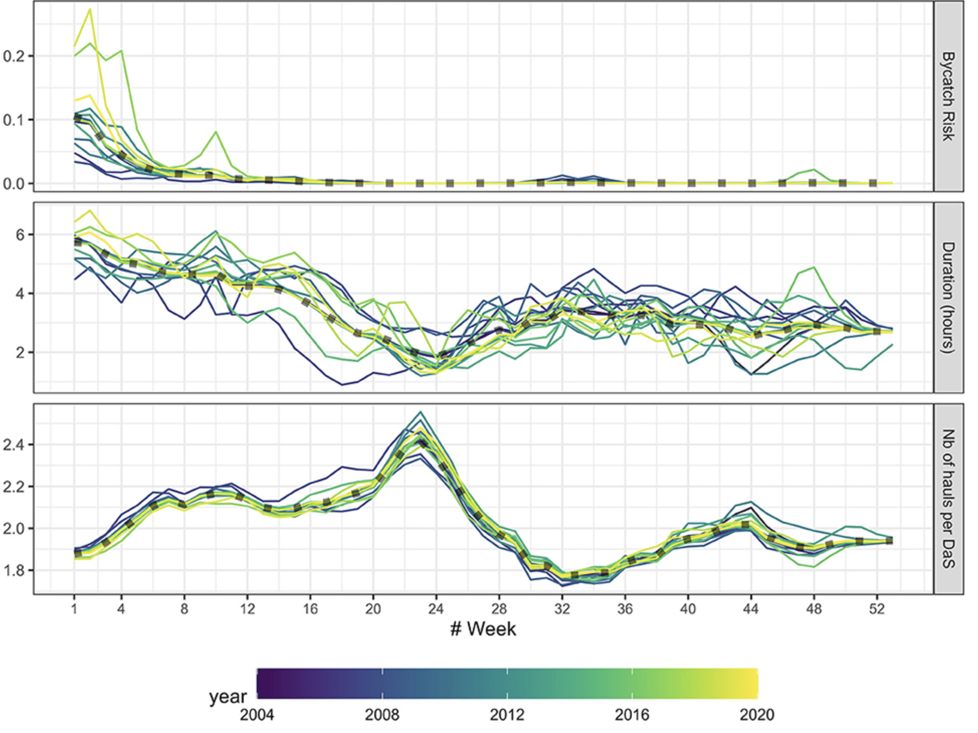
Here is a simulation study using regularized regression with post-stratification to estimate dolphin bycatch from non-representative samples. The Stan code is accessible here.

We’ve used also RRP on a case study with samples from FR where we know that independent observers are preferentially allowed on boat when dolphin bycatch is low (a report is being written at the moment on that, and it will be the second part of the dead dolphin duology for RRP). RRP is giving more plausible estimates in this case.

For those not familiar with the jargon, “bycatch” is “the non-intentional capture or killing of non-target species in commercial or recreational fisheries.”

It’s great to see MRP and Stan being used for all sorts of real problems.

P.S. Authier has an update:

The article has been published and vastly improved thank to peer review. The simulation study is here and the case study is here.

Stan was instrumental in both cases to be able to fit the models.

The model we developed is now used to update estimate bycatch in the Bay of Biscay.

Scholarships for StanCon 2023

(this post is by Charles Margossian)

Applications for the StanCon scholarships are still available. As stated on the conference website:

The purpose of the StanCon scholarship is to make StanCon a more accessible and inclusive event.

Participants who require financial assistance to attend the conference may apply for a scholarship by filling out this formThe StanCon scholarship covers registration for the tutorial and the main conference, as well as local lodging. Scholarships are awarded on a need-base, and prioritize early career scientists, including students and post-docs, and members of underrepresented groups in STEM.

Applications are reviewed on a rolling basis, and scholarships are awarded based on available funds.


Scholarships are made possible by the generosity of our sponsors for the conference: the Washington University in St Louis, Metrum Research Group, and NumFocus. We have already awarded scholarships to highly qualified applicants and we’re very excited to give them the opportunity to attend the conference.

Among the current awardees, we had some well versed Stan users, and also people who are new to Stan. And this is great: the conference gathers experts and also acts as a gateway event, notably via its tutorials, which cover the basics of Stan and more advanced topics.

As a reminder, StanCon is set to take place June 20th – 23rd at the Washington University in St Louis, Missouri.


ChatGPT4 writes Stan code so I don’t have to.

Several months ago I (Phil Price) wrote a Stan model to do some time series forecasting. It took me almost a full day to get it running and debugged. Today I decided to test ChatGPT4, by seeing if it could write a Stan model to give me the same functionality. I have been using ChatGPT to help me with coding, but in the past I’ve used it for little stuff, such as “I have a data frame with column names that all start with mm, and some of the names have ( and ) in them; write a function to remove all of that”. I have just started using it to write entire programs for me, and it looks like it is going to be enormously useful. Below, I present a verbatim transcript of the start of a ChatGPT4 session. At the end I got tired of cutting and pasting — and you would have gotten tired of reading it — but I tell you what happened. And at the very end, I’ll summarize my thoughts on the ChatGPT4 programming experience thus far.


Phil: I have monthly time series data. I want to fit a model to the data (typically from the past five to eight years) and use the model to forecast future values. Let’s call the data y[t]. Here are some things I want to include:
1. Seasonality. If the value in March is high in one year it is probably also high in the following year, and so on for other months. So I want ‘month effects’.
2. Autocorrelation in month effects. The month effect, for a given month of the year, is not iid random. If the March effect is high for several years and then drops a lot, it is more likely to stay low than to jump back up.
3. Local trend. If the value has increased for the past several months it will probably keep increasing, although it might not.
4. Soft constraints. The value of y[t] is very unlikely to fall below a value y_low, or to go above y_high. I don’t want to impose the constraints after the fact. Instead, I want to repel the forecasts from these limits. I want a fairly short-range repulsion, so the forecasts aren’t affected unless they get close to the limits.

Please write a Stan program to do this, and include comments that show where each of those four requirements is implemented.

ChatGPT4: Here’s a Stan program that incorporates seasonality, autocorrelation in month effects, local trend, and soft constraints:

Continue reading

StanCon 2023: deadline for proposals extended!

…. and good news: the proposal deadline for StanCon 2023 has been extended to **April 30th**. We are mostly looking for proposals for talks, themed sessions, and posters:

We are interested in a broad range of topics relevant to the Stan community, including:

– Applications of Bayesian statistics using Stan in all domains

– Software development to support or complement the Stan ecosystem

– Methods for Bayesian modeling, relevant to a broad range of users

– Theoretical insights on common Bayesian methods and models

– Visualization techniques

– Tools for teaching Bayesian modeling.

Proposals are reviewed on a rolling basis. Several talks have already been accepted and added to the schedule, and I’m very excited about the speakers we have so far! Topics include: applications of Stan in numerous fields (healthcare, econometrics, pharmacometrics, ….), interfacing Stan with custom inference algorithms, advances in Bayesian methodology, visualisation and monitoring of MCMC while the Markov chains are running, discussions on Stan/Torsten and Turing.jl and more.

(and this does not include some of the exciting submissions we’ve recently received, although I can’t comment too much…)

There are also some wonderful tutorials lined up. I want to emphasize that a lot of the expertise the community uses to answer questions on the stan forum (https://discourse.mc-stan.org/) is taught during these tutorials.

Here’s a link to the event page https://mc-stan.org/events/stancon2023/ and as always, questions can be addressed to [email protected].

Happy weekend everyone!

StanCon 2023: call for proposals is still open!

This year, we’re bringing back StanCon in person!

StanCon is an opportunity for members of the broader Stan community to come together and discuss applications of Stan, recent developments in Bayesian modeling, and (most importantly perhaps) unsolved problems. The conference attracts field practitioners, software developers, and researchers working on methods and theory. This year’s conference will take place on June 20 – 23 at Washington University in St Louis, Missouri.

The keynote speakers are:

  • Bob Carpenter (Flatiron Institute)
  • John Kruschke (Indiana University)
  • Mariel Finucane (Mathematica Policy Research)
  • Siddhartha Chib (Washington University in St. Louis)

Proposals for talks, sessions and tutorials are due on March 31st (though it looks like we’ll be able to extend the deadline). Posters are accepted on a rolling basis. From the website:

We are interested in a broad range of topics relevant to the Stan community, including:

  • Applications of Bayesian statistics using Stan in all domains
  • Software development to support or complement the Stan ecosystem
  • Methods for Bayesian modeling, relevant to a broad range of users
  • Theoretical insights on common Bayesian methods and models
  • Visualization techniques
  • Tools for teaching Bayesian modeling

Keep in mind that StanCon brings together a diverse audience. Material which focuses on an application should introduce the problem to non-field experts; theoretical insights should be linked to problems modelers are working on, etc.

Parallelization for Markov chain Monte Carlo with heterogeneous runtimes: a case-study on ODE-based models

(this post is by Charles)

Last week, BayesComp 2023 took place in Levi, Finland. The conference covered a broad range of topics in Bayesian computation, with many high quality sessions, talks, and posters. Here’s a link to the talk abstracts. I presented two posters at the event. The first poster was on assessing the convergence of MCMC in the many-short-chains regime. I already blogged about this research (link): here’s the poster and the corresponding preprint.

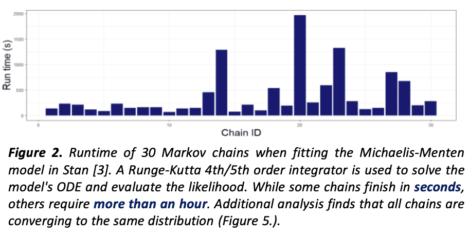
The second poster was also on the topic of running many chains in parallel but in the context of models based on ordinary differential equations (ODEs). This was the outcome of a project led by Stanislas du Ché, during his summer internship at Columbia University. We examined several pharmacometrics models, with likelihoods parameterized by the solution to an ODE. Having to solve an ODE inside a Bayesian model is challenging because the behavior of the ODE can change as the Markov chains journey across the parameter space. An ODE which is easy-to-solve at some point can be incredibly difficult somewhere else. In the past, we analyzed this issue in the illustrative planetary motion example (Gelman et al (2020), Section 11). This is the type of problem where we need to be careful about how we initialize our Markov chains and we should not rely on Stan’s defaults. Indeed, these defaults can start you in regions where your ODE is nearly impossible to solve and completely kill your computation! A popular heuristic is to draw the initial point from the prior distribution. On a related note, we need to construct priors carefully to exclude patently absurd parameter values and (hopefully) parameter values prone to frustrate our ODE solvers.

Even then—and especially if our priors are weakly informative—our Markov chains will likely journey through challenging regions. A common manifestation of this problem is that some chains lag behind because their random trajectories take them through areas that frustrate the ODE solver. Stanislas observed that this problem becomes more acute when we run many chains. Indeed, as we increase the number of chains, the probability that at least some of the chains get “stuck” increases. Then, even when running chains in parallel, the efficiency of MCMC as measured by effective sample size per second (ESS/s) eventually goes down as we add more chains because we are waiting for the slowest chain to finish!

Ok. Well, we don’t want to be punished for throwing more computation at our problem. What if we instead waited for the fastest chains to finish? This is what Stanislas studied by proposing a strategy where we stop the analysis after a certain ESS is achieved, even if some chains are still warming up. An important question is what bias does dropping chains introduce? One concern is that the fastest chains are biased because they fail to explore a region of the parameter space which contains a non-negligible amount of probability mass and where the ODE happens to be more difficult to solve. Stanislas tried to address this problem using stacking (Yao et al 2018), a strategy designed to correct for biased Markov chains. But stacking still assumes all the chains somehow “cover” the region where the probability mass concentrates and, when properly weighted, produce unbiased Monte Carlo estimators.

We may also wonder about the behavior of the slow chains. If the slow chains are close to stationarity, then by excluding them we are throwing away samples which would reduce the variance of our Monte Carlo estimators, however, it’s not worth waiting for these chains to finish if we’ve already achieved the wanted precision. What is more, as Andrew Gelman pointed out to me, slow chains can often be biased, for example if they get stuck in a pathological region during the warmup and never escape this region—as was the case in the planetary motion example. But we can’t expect this to always be the case.

In summary, I like the idea of waiting only for the fastest chains and I think understanding how to do this in a robust manner remains an open question. This work posed the problem and took steps in the right direction. There was a lot of traffic at the poster and I was pleased to see many people at the conference working on ODE-based models.

Haemoglobin blogging

Gavin Band writes:

I wondered what you (or your readers) make of this. Some points that might be of interest:

– The effect we discover is massive (OR > 10).
– The number of data points supporting that estimate is not *that* large (Figure 2).
– it can be thought of as a sort of collider effect – (human and parasite genotypes affecting disease status, which we ascertain on) – though I haven’t figured whether it’s really useful to think of it that way.
– It makes use of Stan! (Albeit only in a relatively minor way in Figure 2).

All in all it’s a pretty striking signal and I wondered what a stats audience make of this – maybe it’s all convincing, or maybe there are things we’ve overlooked or could have done better? I’d certainly be interested in any thoughts…

The linked article is called “The protective effect of sickle cell haemoglobin against severe malaria depends on parasite genotype,” and I have nothing to say about it, as I’ve always found genetics to be very intimidating! But I’ll share with all of you.

“A complete, current, and granular picture of COVID-19 epidemic in the United States”

Bob Carpenter writes:

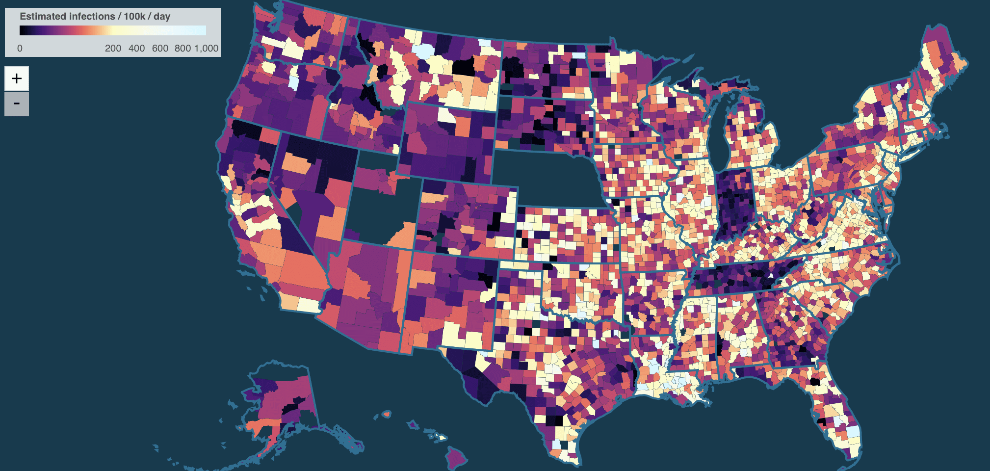
Here’s an app estimating county-level Covid for the US with the uncertainties. The methodology sounds very pragmatic in its combination of
optimization and sampling for hierarchical models.

I like it! And not just because they use Stan.

I just have a few criticisms regarding their displays:

1. I don’t like the color scheme of their map. This thing where they mix in hue changes with intensity changes is just a mess. Not as bad as the notorious rainbow color scheme but not good.

2. I wish they would not list states in alphabetical order: Alabama, Alaska, etc.

If you want a look-up table, that’s fine, but for the main display it’s better to show things that are telling the story.

3. All these graphs look kinda the same. Not identical, but similar. How bout showing the estimated national curve and then for each state showing it relative to the national average?

4. I don’t like this rate-per-100,000 thing. I get that this is standard for epidemiology, but for anyone else (including me), it’s a mess, involving lots of shifting of decimal places in my head. If you want to do the rate per X, why rate per million—this would be a bit easier to follow, no? Or go the other way and just give straight-up percentages. The y-axes for these graphs are labeled 0, 1k, 2k. That’s just 0, 1%, 2%. To me, “1%” is much more clear than “1k” with an implicit “per 100,000.”

5. The x-axes on these time series are a disaster. “12/8, 6/13, 12/22”? What’s that all about? Just give months and years, please! I don’t want to have to decode the damn axis. Baby steps here.

But these are minor comments. Overall it’s an impressive page, and great to see all the data and code there too.

Implementing Laplace approximation in Stan: What’s happening under the hood

Bob Carpenter and I have been talking about implementation of the Laplace approximation (based on mode and curvature of the log posterior density on the unconstrained scale) in Stan. As usual, there are lots of details that I don’t think about until the work is mostly done, and then lots more details that I never think about at all. As a public service, Bob prepared this summary.

Before going on, let me explain that the Laplace approximation is an old idea and a simple idea. Here are some advantages, limitations, and challenges of implementing Laplace:

Advantages of Laplace:
– Relatively cheap to compute, given that we already have a mode-finder in Stan.
– Easy to understand, use, and communicate.
– Works reasonably well in many examples (wherever the posterior can be well approximated by a normal distribution).
– Easy to take draws from the normal approximation, also easy to compute importance ratios and use Pareto-smoothed importance sampling.

Limitations of Laplace:
– Sometimes the normal approx is pretty bad (funnels, multimodal distributions, long tails).
– Sometimes the joint mode is useless or does not even exist (funnels, etc.), in which case the model itself would need to be altered in some way to get a stable mode.

These last two points are kind of obvious, in that the Laplace approximation is hundreds of years old and was the standard approach for Bayesian computation all the way through the 1980s, so if it really did the job, we wouldn’t need Stan at all.

In that case, why implement Laplace in Stan all? The answer: it’s part of workflow. Mode-finding is fast, and we can do a lot of useful model exploration by fitting models fast. And, once you have the mode, a normal approximation centered at the mode can be a useful accessory.

Finally, the challenges of implementing Laplace:
– We can’t easily and generally compute the second-derivative matrix using autodiff, so instead we numerically differentiate the gradients.
– In high dimensions, you’re carrying around a K x K matrix, which can just be too big to handle.
– All the programming details (see below).

Ok, now to Bob’s report:

After our long design back and forth, I [Bob] thought you might be amused to see what happens next on the coding front.

I [Bob] finished writing the C++ code and the tests for Laplace approximation. I’d say it took me around 8 hours total to get it feature complete and tested. It would’ve been faster, but I never wrote anything in the service layer before, so I had to look up all the support functions and test functions, such as how to deal with CSV output from the sample writer. I know C++ pretty well, so that wasn’t a problem, but the assumptions surrounding our code base have gotten very deep and thus are very tough for a directionally challenged person like me to navigate. I thought you might be amused to see what the C++ code for a simple function like this looks like and then what the tests look like, so I’ve appended them. The rest of this note is a description of what the process looks like to get something into Stan.

A change like this requires checking out a new branch of the code from GitHub, doing the modification on that branch, then submitting a pull request to merge that branch back into the development branch of our code. That’s where I’m at right now. We do that so that the development branch of the code always works and is always ready for release and so that we can all work on different parts of the code simultaneously.

After writing the code and the tests are done and the pull request is submitted, the continuous integration kicks off tests that ensure we’ve followed basic coding standards, checks that the changes can be merged into the develop branch without conflicts, and then auto-formats the code and pushes the auto-formatted code back to my branch. Then CI kicks off automatic testing on the formatted branch. The CI steps are what Nick (Nicursor Serban) is maintaining—they run on the Flatiron Institute servers now, so we’re saving a few $K/month in Amazon fees. We test everything on multiple compilers for Windows, Linux, and the Mac. If the integration tests fail (e.g., it won’t compile on Windows or I relied on some undefined behavior that’s different in Linux and on the Mac or at different compilation levels or implementations of arithmetic), then I debug, fix it, and update the pull request and another round of continuous integration kicks off automatically.

Then when tests are passing for my submitted branch, another developer with merge permission (the people listed on our web site) is going to go through all the code and review it. They’ll have requested changes, such as how to write clearer doc or how to make matrix operations faster, or how to use built-in functions rather than a one-off. Then we either discuss the requested changes, or I just make them. Then after the updates, we go back to the top of continuous integration. When the tests pass and all changes are done, it goes back to the original reviewer for another review. This can iterate, but we try not to go multiple cycles of review. When the reviewer is happy, they approve the changes and merge the code in the pull request into the develop branch of the code.

Before it is “in Stan” in a way that you can use it, we have to repeat this entire process for integration into CmdStan. That requires deciding what file formats to use and what the command-line interface is going to look like in terms of arguments and error handling.

CmdStan also requires the CmdStan user’s guide to be updated, which is its own set of updates and pull requests and code review.

Then when it’s merged into CmdStan, we repeat the whole process again for CmdStanPy. That requires defining what the arguments and defaults are going to look like in Python and what the in-memory data structures are going to be and interacting with the formats defined by CmdStan using files and the operating system. That then turns into a pull request that gets reviewed, and hopefully eventually merged. At least the doc for CmdStanPy is in the same repository, so it doesn’t require multiple pull requests.

Then when CmdStanPy is done, everything we did for CmdStanPy gets done again for CmdStanR, but the interfaces might change slightly to match R coding and interface conventions. This is mainly a matter of translation, but it’s just as much code, testing, review, and documentaiton as for CmdStanPy.

Then, the next time a release happens (every 3 to 4 months), the code automatically gets merged from the develop branch into the main branch, and gets included in our release. At this point, we try to write release notes so that users know what has changed version to version.

Anyway, that’s what it means to put something “in Stan” and “in the Stan interfaces”. It’s a lot of work, but there’s really no other choice if we want to keep things stable and we want to keep the state of our development going asynchronously with multiple people working on different parts of the code. By my count we need a pull request and code review for: Stan, CmdStan, CmdStan docs, CmdStanPy, and CmdStanR. It’ll require at least me (basic feature), Mitzi (CmdStan and CmdStanPy) and Jonah (CmdStanR) to be involved, plus three additional people to review the pull requests.

So that’s why I was so insistent during the design discussion to get a sign off from you on what exactly to implement. If it goes all the way to CmdStanR and you’re not happy, we have to go right back to the top of this process and iterate, which is super time consuming, as I’m sure you can imagine given the description.

I’m tired just typing this, but I thought it might help you understand why I’m so obsessed with getting a final design that you are OK with before breaking ground on the code. I’m not at all complaining—just saying that it’s not so trivial to add even a simple algorithm like Laplace approximation.

If it’s just something like a new function to include in Stan, then it’s just a matter of doing a pull request for the math library (C++ code) and a new pull request for the language compiler, stanc (OCaml code) and for the functions reference and optionally the user’s guide. Much easier, but it still requires a lot of complementary skills.

And his code:

=============IMPLEMENTATION===========================

#ifndef STAN_SERVICES_OPTIMIZE_LAPLACE_SAMPLE_HPP
#define STAN_SERVICES_OPTIMIZE_LAPLACE_SAMPLE_HPP

#include <stan/callbacks/interrupt.hpp>
#include <stan/callbacks/logger.hpp>
#include <stan/callbacks/writer.hpp>
#include <stan/math/rev.hpp>
#include <stan/services/error_codes.hpp>
#include <stan/services/util/create_rng.hpp>
#include <string>
#include <type_traits>
#include <vector>

namespace stan {
namespace services {
namespace internal {

template <bool jacobian, typename Model>
void laplace_sample(const Model& model, const Eigen::VectorXd& theta_hat,
   int draws, unsigned int random_seed,
   int refresh, callbacks::interrupt& interrupt,
   callbacks::logger& logger,
   callbacks::writer& sample_writer) {
  if (draws <= 0) {
    throw std::domain_error("Number of draws must be > 0; found draws = "
   + std::to_string(draws));
  }
  
  std::vector<std::string> unc_param_names;
  model.unconstrained_param_names(unc_param_names, false, false);
  int num_unc_params = unc_param_names.size();

  if (theta_hat.size() != num_unc_params) {
    throw::std::domain_error("Specified mode is wrong size; expected "
    + std::to_string(num_unc_params)
    + " unconstrained parameters, but specified mode has size = "
    + std::to_string(theta_hat.size()));
    
  }

  std::vector<std::string> param_tp_gq_names;
  model.constrained_param_names(param_tp_gq_names, true, true);
  size_t draw_size = param_tp_gq_names.size();

  // write names of params, tps, and gqs to sample writer
  std::vector<std::string> names;
  static const bool include_tp = true;
  static const bool include_gq = true;
  model.constrained_param_names(names, include_tp, include_gq);
  names.push_back("log_p");
  names.push_back("log_q");
  sample_writer(names);

  // create log density functor for vars and vals
  std::stringstream log_density_msgs;
  auto log_density_fun
    = [&](const Eigen::Matrix<stan::math::var, -1, 1>& theta) {
    return model.template log_prob<true, jacobian, stan::math::var>(
      const_cast<Eigen::Matrix<stan::math::var, -1, 1>&>(theta),
      &log_density_msgs);
  };

  // calculate inverse negative Hessian's Cholesky factor
  if (refresh > 0) {
    logger.info("Calculating Hessian\n");
  }
  double log_p;  // dummy
  Eigen::VectorXd grad;  // dummy
  Eigen::MatrixXd hessian;
  interrupt();
  math::internal::finite_diff_hessian_auto(log_density_fun, theta_hat, log_p,
  grad, hessian);
  if (refresh > 0) {
    logger.info(log_density_msgs);
    logger.info("\n");
  }

  // calculate Cholesky factor and inverse
  interrupt();
  if (refresh > 0) {
    logger.info("Calculating inverse of Cholesky factor");
    logger.info("\n");
  }
  Eigen::MatrixXd L_neg_hessian = (-hessian).llt().matrixL();
  interrupt();
  Eigen::MatrixXd inv_sqrt_neg_hessian = L_neg_hessian.inverse().transpose();
  interrupt();
  Eigen::MatrixXd half_hessian = 0.5 * hessian;
   
  // generate draws and output to sample writer
  if (refresh > 0) {
    logger.info("Generating draws");
    logger.info("\n");
  }
  boost::ecuyer1988 rng = util::create_rng(random_seed, 0);
  Eigen::VectorXd draw_vec;  // declare draw_vec, msgs here to avoid re-alloc
  for (int m = 0; m < draws; ++m) {
    interrupt();  // allow interpution each iteration
    if (refresh > 0 && m % refresh == 0) {
      logger.info("iteration: ");
      logger.info(std::to_string(m));
      logger.info("\n");
    }
    Eigen::VectorXd z(num_unc_params);
    for (int n = 0; n < num_unc_params; ++n) {
      z(n) = math::std_normal_rng(rng);
    }

    Eigen::VectorXd unc_draw = theta_hat + inv_sqrt_neg_hessian * z;
    double log_p = log_density_fun(unc_draw).val();
    Eigen::VectorXd diff = unc_draw - theta_hat;
    double log_q = diff.transpose() * half_hessian * diff; 
    
    std::stringstream msgs;
    model.write_array(rng, unc_draw, draw_vec, include_tp, include_gq, &msgs);
    if (refresh > 0) {
      logger.info(msgs);
      logger.info("\n");
    }
    std::vector<double> draw(&draw_vec(0), &draw_vec(0) + draw_size);
    draw.push_back(log_p);
    draw.push_back(log_q);
    sample_writer(draw);
  }
}
}  // namespace internal
  
/**
 * Take the specified number of draws from the Laplace approximation
 * for the model at the specified unconstrained mode, writing the
 * draws, unnormalized log density, and unnormalized density of the
 * approximation to the sample writer and writing messages to the
 * logger, returning a return code of zero if successful.
 *
 * Interrupts are called between compute-intensive operations.  To
 * turn off all console messages sent to the logger, set refresh to 0.
 * If an exception is thrown by the model, the return value is
 * non-zero, and if refresh > 0, its message is given to the logger as
 * an error.
 *
 * @tparam jacobian `true` to include Jacobian adjustment for
 * constrained parameters
 * @tparam Model a Stan model
 * @parma[in] m model from which to sample
 * @parma[in] theta_hat unconstrained mode at which to center the
 * Laplace approximation  
 * @param[in] draws number of draws to generate
 * @param[in] random_seed seed for generating random numbers in the
 * Stan program and in sampling  
 * @param[in] refresh period between iterations at which updates are
 * given, with a value of 0 turning off all messages
 * @param[in] interrupt callback for interrupting sampling
 * @param[in,out] logger callback for writing console messages from
 * sampler and from Stan programs
 * @param[in,out] sample_writer callback for writing parameter names
 * and then draws
 * @return a return code, with 0 indicating success
 */
template <bool jacobian, typename Model>
int laplace_sample(const Model& model, const Eigen::VectorXd& theta_hat,
  int draws, unsigned int random_seed,
  int refresh, callbacks::interrupt& interrupt,
  callbacks::logger& logger,
  callbacks::writer& sample_writer) {
  try {
    internal::laplace_sample<jacobian>(model, theta_hat, draws, random_seed,
      refresh, interrupt, logger,
      sample_writer);
    return error_codes::OK;
  } catch (const std::exception& e) {
    if (refresh >= 0) {
      logger.error(e.what());
      logger.error("\n");
    }
  } catch (...) {
    if (refresh >= 0) {
      logger.error("unknown exception during execution\n");
    }
  }
  return error_codes::DATAERR;
}
}  // namespace services
}  // namespace stan
  
#endif

==========================TEST CASE====================
#include <boost/algorithm/string.hpp>
#include <gtest/gtest.h>
#include <stan/callbacks/stream_logger.hpp>
#include <stan/callbacks/stream_writer.hpp>
#include <stan/io/dump.hpp>
#include <stan/io/empty_var_context.hpp>
#include <stan/io/stan_csv_reader.hpp>
#include <stan/services/error_codes.hpp>
#include <stan/services/optimize/laplace_sample.hpp>
#include <test/test-models/good/services/multi_normal.hpp>
#include <test/unit/services/instrumented_callbacks.hpp>
#include <test/unit/util.hpp>
#include <cmath>
#include <iostream>
#include <vector>

class ServicesLaplaceSample: public ::testing::Test {
 public:
  ServicesLaplaceSample() : logger(msgs, msgs, msgs, msgs, msgs) { }

  void SetUp() {
    stan::io::empty_var_context var_context;
    model = new stan_model(var_context);  // typedef from multi_normal.hpp
  }

  void TearDown() { delete model; }

  stan_model* model;
  std::stringstream msgs;
  stan::callbacks::stream_logger logger;
  stan::test::unit::instrumented_interrupt interrupt;
};

TEST_F(ServicesLaplaceSample, values) {
  Eigen::VectorXd theta_hat(2);
  theta_hat << 2, 3;
  int draws = 50000;  // big to enable mean, var & covar test precision
  unsigned int seed = 1234;
  int refresh = 1;
  std::stringstream sample_ss;
  stan::callbacks::stream_writer sample_writer(sample_ss, "");
  int return_code = stan::services::laplace_sample<true>(*model, theta_hat,
     draws, seed, refresh, interrupt, logger, sample_writer);
  EXPECT_EQ(stan::services::error_codes::OK, return_code);
  std::string samples_str = sample_ss.str();
  EXPECT_EQ(2, count_matches("y", samples_str));
  EXPECT_EQ(1, count_matches("y.1", samples_str));
  EXPECT_EQ(1, count_matches("y.2", samples_str));
  EXPECT_EQ(1, count_matches("log_p", samples_str));
  EXPECT_EQ(1, count_matches("log_q", samples_str));

  std::stringstream out;
  stan::io::stan_csv draws_csv = stan::io::stan_csv_reader::parse(sample_ss, &out);

  EXPECT_EQ(4, draws_csv.header.size());
  EXPECT_EQ("y[1]", draws_csv.header[0]);
  EXPECT_EQ("y[2]", draws_csv.header[1]);
  EXPECT_EQ("log_p", draws_csv.header[2]);
  EXPECT_EQ("log_q", draws_csv.header[3]);

  Eigen::MatrixXd sample = draws_csv.samples;
  EXPECT_EQ(4, sample.cols());
  EXPECT_EQ(draws, sample.rows());
  Eigen::VectorXd y1 = sample.col(0);
  Eigen::VectorXd y2 = sample.col(1);
  Eigen::VectorXd log_p = sample.col(2);
  Eigen::VectorXd log_q = sample.col(2);

  // because target is normal, laplace approx is exact
  for (int m = 0; m < draws; ++m) {
    EXPECT_FLOAT_EQ(0, log_p(m) - log_q(m));
  }

  // expect mean draws to be location params +/0 MC error
  EXPECT_NEAR(2, stan::math::mean(y1), 0.05);
  EXPECT_NEAR(3, stan::math::mean(y2), 0.05);

  double sum1 = 0;
  for (int m = 0; m < draws; ++m) {
    sum1 += std::pow(y1(m) - 2, 2);
  }
  double var1 = sum1 / draws;
  EXPECT_NEAR(1, var1, 0.05);

  double sum2 = 0;
  for (int m = 0; m < draws; ++m) {
    sum2 += std::pow(y2(m) - 3, 2);
  }
  double var2 = sum2 / draws;
  EXPECT_NEAR(1, var2, 0.05);

  double sum12 = 0;
  for (int m = 0; m < draws; ++m) {
    sum12 += (y1(m) - 2) * (y2(m) - 3);
  }
  double cov = sum12 / draws;
  EXPECT_NEAR(0.8, cov, 0.05);
}

TEST_F(ServicesLaplaceSample, wrongSizeModeError) {
  Eigen::VectorXd theta_hat(3);
  theta_hat << 2, 3, 4;
  int draws = 10;
  unsigned int seed = 1234;
  int refresh = 1;
  std::stringstream sample_ss;
  stan::callbacks::stream_writer sample_writer(sample_ss, "");
  int RC = stan::services::laplace_sample<true>(*model, theta_hat, draws, seed, refresh, interrupt, logger, sample_writer);
  EXPECT_EQ(stan::services::error_codes::DATAERR, RC);
}
TEST_F(ServicesLaplaceSample, nonPositiveDrawsError) {
  Eigen::VectorXd theta_hat(2);
  theta_hat << 2, 3;
  int draws = 0;
  unsigned int seed = 1234;
  int refresh = 1;
  std::stringstream sample_ss;
  stan::callbacks::stream_writer sample_writer(sample_ss, "");
  int RC = stan::services::laplace_sample<true>(*model, theta_hat, draws, seed, refresh, interrupt, logger, sample_writer);
  EXPECT_EQ(stan::services::error_codes::DATAERR, RC);
}

Free Bayesian Data Analysis course

We’re organizing a free Bayesian Data Analysis course targeted for Global south and other underrepresented groups. This is currently the third rendition of the BDA GSU course. Please see more information and the link to the registration form at the course web page.

The course is based on BDA3 book and BDA course at Aalto. All course material is freely available.

This is not the easiest Bayes course. The registration form requires you to answer some prerequisite questions. The web page has recommendations for easier material.

As all the material is free, you can choose to study at your own pace. We recommend registering and following the common schedule to benefit from the support of your peers and TAs.

If you want to volunteer to be a TA for the course, the course web page has also a link to TA registration.

The head TA is Meenal Jhajharia who did great job also in 2022.

The course is supported by Stan governing body, Numfocus, and Eduflow is supporting us by providing a free license of Peergrade tool.

Our first in-person StanCon since 2019 will be held in Washington University in St. Louis!

Our first in-person StanCon since 2019 will be held in Washington University in St. Louis. Registration and schedule coming soon!

Tutorials and workshops: Tuesday and Wednesday, June 20-21, 2023.

Conference: Thursday and Friday, June 22-23, 2023.

Tutorials: we’re seeking proposals for half-day or full-day tutorials. These can either be focused on foundations of Stan programming and Bayesian inference or advanced topics that can be for a niche audience. Proposals must describe the content and objectives of the tutorial.

Contributed talks: if you’d like to present your work at StanCon 2023, we’re looking for people to talk either in the general session or poster session.
If you have any questions or are considering submitting a proposal, feel free to reach out to [email protected].

Sponsorship: We can’t do this without the support of generous sponsors that support our events! If you’re interested in sponsoring StanCon, let’s talk! ([email protected]).

More details can be found on the Stan Forums.

The conference is organized by Debashis Mondal (Washington University in St. Louis), Eric Ward (University of Washington & NOAA), Charles Margossian (Flatiron Institute), Vianey Leos Barajas (University of Toronto), and Yi Zhang (Sage Therapeutics, Inc). The affiliations of the organizers already indicate the mix of Stan users and developers in academia, business, nonprofits, and government.

Some previous StanCon materials are here.

Bayesian geomorphology

John “not the Jaws guy” Williams points us to this article by Oliver Korup which begins:

The rapidly growing amount and diversity of data are confronting us more than ever with the need to make informed predictions under uncertainty. The adverse impacts of climate change and natural hazards also motivate our search for reliable predictions. The range of statistical techniques that geomorphologists use to tackle this challenge has been growing, but rarely involves Bayesian methods. Instead, many geomorphic models rely on estimated averages that largely miss out on the variability of form and process. Yet seemingly fixed estimates of channel heads, sediment rating curves or glacier equilibrium lines, for example, are all prone to uncertainties. Neighbouring scientific disciplines such as physics, hydrology or ecology have readily embraced Bayesian methods to fully capture and better explain such uncertainties, as the necessary computational tools have advanced greatly. The aim of this article is to introduce the Bayesian toolkit to scientists concerned with Earth surface processes and landforms, and to show how geomorphic models might benefit from probabilistic concepts. I briefly review the use of Bayesian reasoning in geomorphology, and outline the corresponding variants of regression and classification in several worked examples.

Cool! It’s good to see Bayesian ideas in different scientific fields. And they use Stan. I also like that they have graphs of data and fitted models.

Research fellow, postdoc, and doctoral student positions at Aalto University, Finland

We’re looking for research fellows, postdocs, and doctoral students for projects in

  • Bayesian workflows for iterative model building and networks of models (Proj. 7, Aalto University)
  • Evaluating and improving posterior inference for difficult posteriors
    (Proj. F9, FCAI/Aalto/Helsinki with Prof. Arto Klami)
  • Workflows for better priors (Proj. F19, FCAI/Aalto/Helsinki with Prof. Arto Klami)

See the abstracts below.

There are also many other topics in probabilistic modeling, ML, and AI at Aalto University and University of Helsinki

All topics and how to apply at

You can ask me (Aki) for more information

Aalto University and University Helsinki have strong Bayesian/ML/AI community. We contribute to open source software packages like Stan and ArviZ. Aalto pays postdocs well compared to many other countries. We have plenty of travel funds. Finland is a great place for living, with or without family. It is a safe, politically stable and well-organized society, where equality is highly valued and corruption is low. Extensive social security supports people in all situations of life. Occupational and national public healthcare in Finland are great and free. You can manage in work and everyday life well with English (no need to learn Finnish unless you want to). Finland has been ranked as the happiest country in the world in 2018–2021.

Topic: Bayesian workflows for iterative model building and networks of models

We formalize and develop theory and diagnostics for iterative Bayesian model building. The practical workflow recommendations and diagnostics guide the modeller through the appropriate steps to ensure safe iterative model building, or indicate when the modeler is likely to be in the danger zone.

Topic: Evaluating and improving posterior inference for difficult posteriors

Both MCMC and distributional approximations often struggle to handle complex posteriors, but we lack good tools for understanding how and why. We study diagnostics for identifying the nature of the computational difficulty, e.g. whether the difficulty is caused by narrow funnels or strong curvature. We also develop improved inference algorithms, e.g. via automated and semi-automated transformations.

Topic: Workflows for better priors

Bayesian models rely on prior distributions that encode knowledge about the problem, but specifying good priors is often difficult in practice. We are working on multiple fronts on making it easier, with contributions to e.g. prior elicitation, prior diagnostics, prior checking, and specification of priors in predictive spaces.

Update 4 – World Cup Qatar 2022 predictions (semifinals and winning probabilities)

Time for our last update! Qatar 2022 World Cup is progressing fast, and only four teams – Argentina, France, Croatia and Morocco – are still in contention for the final victory. Who will be the winner on December 18th? Is our model better than the Paul the Octopus, an almost perfect oracle during World Cup 2010?

Semifinals predictions

We report in the table below the posterior predictive match probabilities from our DIBP model – get a look also here and here for other updates – for the two semifinals planned for Tuesday, December 13 and Wednesday, December 14, Argentina-Croatia and France-Morocco, respectively. We also report the usual ppd ‘chessboard plots’ for the exact outcomes in gray-scale color.

Notes: ‘mlo’ in the table denotes the ‘most likely result’ , whereas darker regions in the plots correspond to more likely results. The first team listed in each sub-title is the ‘favorite’ (x-axis), whereas the second team is the ‘underdog’ (y-axis). The 2-way grid displays the 2 held-out matches in such a way that the closest match appears in the left panel of the grid, whereas the most unbalanced match (‘blowout’) appears in the right panel. 


France and Argentina seem clearly ahead against Croatia and Morocco, respectively.  Anyway, underdogs  such as Morocco have a non-negligible chance – approximately 35% – to beat France and advance to the final: consider that  Morocco got two ‘clean-sheets‘ in the round of 16 and quarter of finals matches, against Spain and Portugal, respectively!   Croatia already achieved the final four years ago, so maybe it should not be considered as a pure underdog…and Luka Modric, the Croatia’s captain, is still one of the best players in the world.

Note: keep in mind that the above predictions refer to the ‘regular’ times, not to the extra times! Anyway, to get an approximated probability to advance to the final, say for the favorite team, one could compute: favorite probability + 0.5*draw probability. The same could be done for the underdog team. In such a way, with no further assumptions we assume that the draw probability within the regular times is equally split between the two teams in the eventual extra-times. 

World Cup winning probabilities

We also provide some World Cup winning probabilities for the four teams, based on some forward simulations of the tournament.

The results are somehow surprising! Unlike for what happens for the majority of the bookies, Argentina has the highest chances to win the World Cup. France comes at the second place, whereas Morocco is the underdog, with only the 8% probability to become the World Cup winner.

Full code and details

You find the complete results, R code and analysis here. Some preliminary notes and model limitations can be found here. And use the footBayes package!

Final considerations

We had a lot of fun with these World Cup predictions, we guess this has been a good and challenging statistical application. To summarize, the average of the correct probabilities, i.e. the average of the model probabilities for the actually observed outcomes, is 0.41, whereas the pseudo R-squared is 0.36 (up to the quarter of finals matches).

BridgeStan: Stan model log densities, gradients, Hessians, and transforms in R, Python, and Julia

We’re happy to announce the official 1.0.0 release of BridgeStan.

What is BridgeStan?

From the documentation:

BridgeStan provides efficient in-memory access through Python, Julia, and R to the methods of a Stan model, including log densities, gradients, Hessians, and constraining and unconstraining transforms.

BridgeStan should be useful for developing algorithms and deploying applications. It connects to R and Python through low-level foreign function interfaces (.C and ctypes, respectively) and is thus very performant and portable. It is also easy to install and keep up to date with Stan releases. BridgeStan adds the model-level functionality from RStan/PyStan that is not implemented in CmdStanR/CmdStanPy.

Documentation and source code

Detailed forum post

Here’s a post on the Stan forums with much more detail:

Among other things, it describes the history and relations to other Stan-related projects. Edward Roualdes started the project in order to access Stan models through Julia, then Brian Ward and I (mostly Brian!) helped Edward finish it, with some contributions from Nicholas Siccha and Mitzi Morris.

Update 3 – World Cup Qatar 2022 predictions (round of 16)

World Cup 2022 is progressing, many good matches and much entertainment. Time then for World Cup 2022 predictions of the round of 16 matches from our DIBP model  – here the previous update. In the group stage matches the average of the model probabilities for the actual final results was about 0.52.

Here there are the posterior predictive match probabilities for the held-out matches of the Qatar 2022 round of 16 to be played from December 3rd to December 6th, along with some ppd ‘chessboard plots’ for the exact outcomes in gray-scale color – ‘mlo’ in the table denotes the ‘most likely result’ , whereas darker regions in the plots correspond to more likely results. In the plots below, the first team listed in each sub-title is the ‘favorite’ (x-axis), whereas the second team is the ‘underdog’ (y-axis). The 2-way grid displays the 8 held-out matches in such a way that closer matches appear at the top-left of the grid, whereas more unbalanced matches (‘blowouts’) appear at the bottom-right.  The matches are then ordered from top-left to bottom-right in terms of increasing winning probability for the favorite teams. The table reports instead the matches according to a chronological order.

Apparently, Brazil is highly favorite against South Korea, and Argentina seems much ahead against Australia, whereas much balance is predicted for Japan-Croatia, Netherlands-United States and Portugal-Switzerland. Note: take in consideration that these probabilities refer to the regular times, then within the 90 minutes. The model does not capture supplementary times probabilities.

You find the complete results, R code and analysis here. Some preliminary notes and model limitations can be found here.

Next steps: we’ll update the predictions for the quarter of finals. We are still discussing about the possibility to report some overall World Cup winning probabilities, even though I am personally not a huge fan of these ahead-predictions (even coding this scenario is not straightforward…!). However, we know those predictions could be really amusing for fans, so maybe we are going to report them after the round of 16. We also could post some pp checks for the model and more predictive performance measures.

Stay tuned!

A different Bayesian World Cup model using Stan (opportunity for model checking and improvement)

Maurits Evers writes:

Inspired by your posts on using Stan for analysing football World Cup data here and here, as well as the follow-up here, I had some fun using your model in Stan to predict outcomes for this year’s football WC in Qatar. Here’s the summary on Netlify. Links to the code repo on Bitbucket are given on the website.

Your readers might be interested in comparing model/data/assumptions/results with those from Leonardo Egidi’s recent posts here and here.

Enjoy, soccerheads!

P.S. See comments below. Evers’s model makes some highly implausible predictions and on its face seems like it should not be taken seriously. From the statistical perspective, the challenge is to follow the trail of breadcrumbs and figure out where the problems in the model came from. Are they from bad data? A bug in the code? Or perhaps a flaw in the model so that the data were not used in the way that were intended? One of the great things about generative models is that they can be used to make lots and lots of predictions, and this can help us learn where we have gone wrong. I’ve added a parenthetical to the title of this post to emphasize this point. Also good to be reminded that just cos a method uses Bayesian inference, that doesn’t mean that its predictions make any sense! The output is only as good as its input and how that input is processed.

Update 2 – World Cup Qatar 2022 Predictions with footBayes/Stan

Time to update our World Cup 2022 model!

The DIBP (diagonal-inflated bivariate Poisson) model performed very well in the first match-day of the group stage in terms of predictive accuracy – consider that the ‘peudo R-squared’, namely the geometric mean of the probabilities assigned from the model to the ‘true’ final match results, is about 0.4, whereas, on average, the main bookmakers got 0.36.

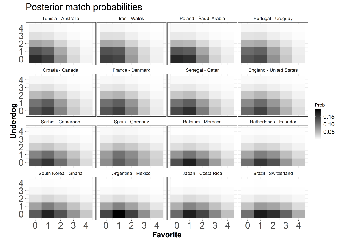
It’s now time to re-fit the model after the first 16 group stage games with the footBayes R package and obtain the probabilistic predictions for the second match-day. Here there are the posterior predictive match probabilities for the held-out matches of the Qatar 2022 group stage played from November 25th to November 28th, along with some ppd ‘chessboard plots’ for the exact outcomes in gray-scale color – ‘mlo’ in the table denotes the ‘most likely result’ , whereas darker regions in the plots correspond to more likely results.

Plot/table updates: (see Andrew’ suggestions from the previous post, we’re still developing these plots to improve their appearance, see below some more notes). In the plots below, the first team listed in each sub-title is the ‘favorite’ (x-axis), whereas the second team is the ‘underdog’ (y-axis). The 2-way grid displays the 16 held-out matches in such a way that closer matches appear at the top-left of the grid, whereas more unbalanced matches (‘blowouts’) appear at the bottom-right.  The matches are then ordered from top-left to bottom-right in terms of increasing winning probability for the favorite teams. The table reports instead the matches according to a chronological order.

The most unbalanced game seems Brazil-Switzerland, where the Brazil is the favorite team with an associated winning probability about 71%. The closest game seems Iran-Wales – Iran just won with two goals of margin scored in the last ten minutes! – whereas France is given only 44% probability of winning against Denmark. Argentina seems to be ahead against Mexico, whereas Spain seems to have a non-negligible advantage in the match against Germany.

Another predictive note: Regarding ‘most-likely-outcomes’ (mlo here above), the model ‘guessed’ 4 ‘mlo’ out of 16 in the previous match-day.

You find the complete results, R code and analysis here.

Some more technical notes/suggestions about the table and the plots above:

  • We replaced ‘home’ and ‘away’ by ‘favorite’ and ‘underdog’.
  • I find difficult to handle ‘xlab’ and ‘ylab’ in faceted plots with ggplot2! (A better solution could be in fact to directly put the team names on each of the axes of the sub-plots).
  • The occurrence ‘4’ actually stands for ‘4+’, meaning that it captures the probability of scoring ‘4 or more goals’ (I did not like the thick ‘4+’ in the plot, for this reason we just set ‘4’, however we could improve this).
  • We could consider adding some global ‘x’ and ‘y’-axes with probability margins between underdog and  favorite. Thus, for Brazil-Switzerland, we should have a thick on the x-axis at approximately 62%, whereas for Iran-Wales at 5%.

For other technical notes and model limitations check the previous post.

Next steps: we are going to update the predictions for the third match-day and even compute some World Cup winning probabilities through a ahead-simulation of the whole tournament.

Stay tuned!