Rosenthal’s textbook: A First Look at Rigorous Probability Theory

I’ve never taken a stats class. I was a math major, but dropped stats after I got appendicitis because I didn’t want to drop abstract algebra or computability theory. So here I am 40 years later trying to write up some more formal notes on probability theory and Markov chain Monte Carlo methods (MCMC) and finding myself in need of a gentle intro to probability theory that defines things rigorously. Jeffrey S. Rosenthal’s 2006 book A First Look at Rigorous Probability Theory is just what I needed. Despite not being very good at continuous math as an undergrad, I would have loved this book as it’s largely algebraic, topological, and set-theoretic in approach rather than relying on in-depth knowledge of real analysis or matrix algebra. Even the examples are chosen to be simple rather than being designed for Ph.D.s in math, and even include a lot of basic analysis results like constructing uncountable, unmeasurable sets.

This is not the final book you’ll need on your way to becoming a measure theorist. For example, it never discusses Radon-Nikodym derivatives to unify the theory of pdfs. It doesn’t really get into stochastic processes beyond a high-level discussion of Brownian motion. It does cover the basic theory of general state space, time-homogeneous Markov chains in a few pages (why I was reading it), but that’s just scratching the surface of Rosenthal and Roberts’ general state-space MCMC paper which is dozens of pages long in much finer print.

One of the best features of the book is that it’s both short and packed with meaningful examples. Rosenthal was quite selective in eliminating unnecessary fluff and sticking to the through line of introducing the main ideas. Most of the texts in this area just can’t resist all kinds of side excursions, examples which bring in all sorts of Ph.D. level math. That can be good if you need breadth and depth, but Rosenthal’s approach is superior for a first, broad introduction to the field.

In summary: 5/5 stars.

We were measuring the speed of Stan incorrectly—it’s faster than we thought in some cases due to antithetical sampling

Aki points out that in cases of antithetical sampling, our effective sample size calculations were unduly truncated above at the number of iterations. It turns out the effective sample size can be greater than the number of iterations if the draws are anticorrelated. And all we really care about for speed is effective sample size per unit time.

NUTS can be antithetical

The desideratum for a sampler Andrew laid out to Matt was to maximze expected squared transition distance. Why? Because that’s going to maximize effective sample size. (I still hadn’t wrapped my head around this when Andrew was laying it out.) Matt figured out how to achieve this goal by building an algorithm that simulated the Hamiltonian forward and backward in time at random, doubling the time at each iteration, and then sampling from the path with a preference for the points visited in the final doubling. This tends to push iterations away from their previous values. In some cases, it can lead to anticorrelated chains.

Removing this preference for the second half of the chains drastically reduces NUTS’s effectiveness. Figuring out how to include it and satisfy detailed balance was one of the really nice contributions in the original NUTS paper (and implementation).

Have you ever seen 4000 as the estimated n_eff in a default Stan run? That’s probably because the true value is greater than 4000 and we truncated it.

The fix is in

What’s even cooler is that the fix is already in the pipeline and it just happens to be Aki’s first C++ contribution. Here it is on GitHub:

Aki’s also done simulations, so the new version is actually better calibrated as far as MCMC standard error goes (posterior standard deviation divided by the square root of the effective sample size).

A simple example

Consider three Markov processes for drawing a binary sequence y[1], y[2], y[3], …, where each y[n] is in { 0, 1 }. Our target is a uniform stationary distribution, for which each sequence element is marginally uniformly distributed,

Pr[y[n] = 0] = 0.5     Pr[y[n] = 1] = 0.5  

Process 1: Independent. This Markov process draws each y[n] independently. Whether the previous state is 0 or 1, the next state has a 50-50 chance of being either 0 or 1.

Here are the transition probabilities:

Pr[0 | 1] = 0.5   Pr[1 | 1] = 0.5
Pr[0 | 0] = 0.5   Pr[1 | 0] = 0.5

More formally, these should be written in the form

Pr[y[n + 1] = 0 | y[n] = 1] = 0.5

For this Markov chain, the stationary distribution is uniform. That is, some number of steps after initialization, there’s a probability of 0.5 of being in state 0 and a probability of 0.5 of being in state 1. More formally, there exists an m such that for all n > m,

Pr[y[n] = 1] = 0.5

The process will have an effective sample size exactly equal to the number of iterations because each state in a chain is independent.

Process 2: Correlated. This one makes correlated draws and is more likely to emit sequences of the same symbol.

Pr[0 | 1] = 0.01   Pr[1 | 1] = 0.99
Pr[0 | 0] = 0.99   Pr[1 | 0] = 0.01

Nevertheless, the stationary distribution remains uniform. Chains drawn according to this process will be slow to mix in the sense that they will have long sequences of zeroes and long sequences of ones.

The effective sample size will be much smaller than the number of iterations when drawing chains from this process.

Process 3: Anticorrelated. The final process makes anticorrelated draws. It’s more likely to switch back and forth after every output, so that there will be very few repeating sequences of digits.

Pr[0 | 1] = 0.99   Pr[1 | 1] = 0.01
Pr[0 | 0] = 0.01   Pr[1 | 0] = 0.99

The stationary distribution is still uniform. Chains drawn according to this process will mix very quickly.

With an anticorrelated process, the effective sample size will be greater than the number of iterations.

Visualization

If I had more time, I’d simulate, draw some traceplots, and also show correlation plots at various lags and the rate at which the estimated mean converges. This example’s totally going in the Coursera course I’m doing on MCMC, so I’ll have to work out the visualizations soon.
Interactive visualizations of sampling and GP regression

You really don’t want to miss Chi Feng‘s absolutely wonderful interactive demos.

(1) Markov chain Monte Carlo sampling

I believe this is exactly what Andrew was asking for a few Stan meetings ago:

This tool lets you explore a range of sampling algorithms including random-walk Metropolis, Hamiltonian Monte Carlo, and NUTS operating over a range of two-dimensional distributions (standard normal, banana, donut, multimodal, and one squiggly one). You can control both the settings of the algorithms and the settings of the visualizations. As you run it, it even collects the draws into a sample which it summarizes as marginal histograms.

Source code

The demo is implemented in Javascript with the source code on Chi Feng’s GitHub organization:

Wish list

  1. 3D (glasses or virtual reality headset)
  2. multiple chains in parallel
  3. scatterplot breadcrumbs
  4. Gibbs sampler
  5. Ensemble samplers
  6. User-pluggable densities (Andrew really wants this for Stan where you’d choose two dimensions of N to visualize)

(2) Gaussian Process visualization

This one’s also really elegant.

It lets you lay down a few points and fit a 1D GP. It lets you choose kernel and hperparameters, and even sample regression functions from it conditioned on the data you provide.

Wish list

  1. 3D (OK, I’m obssesed, but this one would be great on a 2D grid with a 3D visualization of a GP being fit)
  2. Estimating hyperparameters (didn’t seem like it was doing this—may be a bit challenging for Javascript!)

Source code

ShinyStan v2.0.0

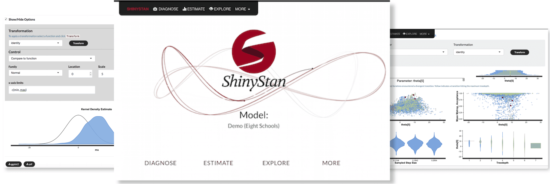
For those of you not familiar with ShinyStan, it is a graphical user interface for exploring Stan models (and more generally MCMC output from any software). For context, here’s the post on this blog first introducing ShinyStan (formerly shinyStan) from earlier this year.

shinystan_images

ShinyStan v2.0.0 released

ShinyStan v2.0.0 is now available on CRAN. This is a major update with a new look and a lot of new features. It also has a new(ish) name: ShinyStan is the app/GUI and shinystan the R package (both had formerly been shinyStan for some reason apparently not important enough for me to remember). Like earlier versions, this version has enhanced functionality for Stan models but is compatible with MCMC output from other software packages too.

You can install the new version from CRAN like any other package:

install.packages("shinystan")

If you prefer a version with a few minor typos fixed you can install from Github using the devtools package:

devtools::install_github("stan-dev/shinystan", build_vignettes = TRUE)

(Note: after installing the new version and checking that it works we recommend removing the old one by running remove.packages(“shinyStan”).)

If you install the package and want to try it out without having to first fit a model you can launch the app using the preloaded demo model:

library(shinystan)
launch_shinystan_demo()

Notes

This update contains a lot of changes, both in terms of new features added, greater UI stability, and an entirely new look. Some release notes can be found on GitHub and there are also some instructions for getting started on the ShinyStan wiki page. Here are two highlights:

  • The new interactive diagnostic plots for Hamiltonian Monte Carlo. In particular, these are designed for models fit with Stan using NUTS (the No-U-Turn Sampler).

    Diagnostics screenshot Diagnostics screenshotshinystan_diagnostics3

  • The deploy_shinystan function, which lets you easily deploy ShinyStan apps for your models to RStudio’s ShinyApps hosting service. Each of your apps (i.e. each of your models) will have a unique URL. To use this feature please also install the shinyapps package: devtools::install_github("rstudio/shinyapps").

The plan is to release a minor update with bug fixes and other minor tweaks in a month or so. So if you find anything we should fix or change (or if you have any other suggestions) we’d appreciate the feedback.

A Stan is Born

Stan 1.0.0 and RStan 1.0.0

It’s official. The Stan Development Team is happy to announce the first stable versions of Stan and RStan.

What is (R)Stan?

Stan is an open-source package for obtaining Bayesian inference using the No-U-Turn sampler, a variant of Hamiltonian Monte Carlo. It’s sort of like BUGS, but with a different language for expressing models and a different sampler for sampling from their posteriors.

RStan is the R interface to Stan.

Stan Home Page

Stan’s home page is: http://mc-stan.org/

It links everything you need to get started running Stan from the command line, from R, or from C++, including full step-by-step install instructions, a detailed user’s guide and reference manual for the modeling language, and tested ports of most of the BUGS examples.

Peruse the Manual

If you’d like to learn more, the Stan User’s Guide and Reference Manual is the place to start.

Learning Differential Geometry for Hamiltonian Monte Carlo

You can get a taste of Hamiltonian Monte Carlo (HMC) by reading the very gentle introduction in David MacKay’s general text on information theory:

Follow this up with Radford Neal’s much more thorough introduction to HMC:

  • Neal, R. 2011. MCMC Using Hamiltonian Dynamics. In Brooks, Gelman, Jones and Meng, eds., Handbook of Markov Chain Monte Carlo. Chapman and Hall/CRC Press.

To understand why HMC works and set yourself on the path to understanding generalizations like Riemann manifold HMC, you’ll need to know a bit about differential geometry. I really liked the combination of these two books:

  • Magnus, J. R. and H. Neudecker. 2007. Matrix Differential Calculus with Application in Statistics and Econometrics. 3rd Edition. Wiley?

and

As a bonus, Magnus and Neudecker also provide an excellent introduction to matrix algebra and real analysis before mashing them up. The question mark after “Wiley” is due to the fact that the preface says that the third-edition is self-published and copyright the authors and and available from the first author’s home page. It’s no longer available on Magnus’s home page, nor is it available for sale by Wiley. It can be found in PDF form on the web, though; try Googling [matrix differential calculus magnus].