Time Series Forecasting: futile but necessary. An example using electricity prices.

This post is by Phil Price, not Andrew.

I have a client company that owns refrigerated warehouses around the world. A refrigerated warehouse is a Costco-sized building that is kept very cold; 0 F is a common setting in the U.S. (I should ask what they do in Europe). As you might expect, they have an enormous electric bill — the company as a whole spends around a billion dollars per year on electricity — so they are very interested in the cost of electricity. One decision they have to make is: how much electricity, if any, should they purchase in advance? The alternative to purchasing in advance is paying the “real-time” electricity price. On average, if you buy in advance you pay a premium…but you greatly reduce the risk of something crazy happening. What do I mean by ‘crazy’? Take a look at the figure below. This is the monthly-average price per Megawatt-hour (MWh) for electricity purchased during the peak period (weekday afternoons and evenings) in the area around Houston, Texas. That big spike in February 2021 is an ice storm that froze a bunch of wind turbines and also froze gas pipelines — and brought down some transmission lines, I think — thus leading to extremely high electricity prices. And this plot understates things, in a way, by averaging over a month: there were a couple of weeks of fairly normal prices that month, and a few days when the price was over $6000/MWh.

Monthly-mean peak-period (weekday afternoon) electricity price, in dollars per megawatt-hour, in Texas.

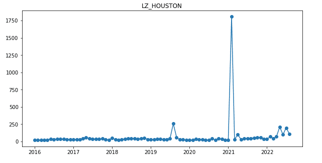
If you buy a lot of electricity, a month when it costs 20x as much as you expected can cause havoc with your budget and your profits. One way to avoid that is to buy in advance: a year ahead of time, or even a month ahead of time, you could have bought your February 2021 electricity for only a bit more than electricity typically costs in Texas in February. But events that extreme are very rare — indeed I think this is the most extreme spike on record in the whole country in at least the past thirty years — so maybe it’s not worth paying the premium that would be involved if you buy in advance, month after month and year after year, for all of your facilities in the U.S. and Europe. To decide how much electricity to buy in advance (if any) you need at least a general understanding of quite a few issues: how much electricity do you expect to need next month, or in six months, or in a year; how much will it cost to buy in advance; how much is it likely to cost if you just wait and buy it at the time-of-use rate; what’s the chance that something crazy will happen, and, if it does, how crazy will the price be; and so on.

Continue reading

Stan Weekly Roundup, 30 June 2017

TM version of logoHere’s some things that have been going on with Stan since the last week’s roundup

  • Stan® and the logo were granted a U.S. Trademark Registration No. 5,222,891 and a U.S. Serial Number: 87,237,369, respectively. Hard to feel special when there were millions of products ahead of you. Trademarked names are case insensitive and they required a black-and-white image, shown here.

  • Peter Ellis, a data analyst working for the New Zealand government, posted a nice case study, State-space modelling of the Australian 2007 federal election. His post is intended to “replicate Simon Jackman’s state space modelling [from his book and pscl package in R] with house effects of the 2007 Australian federal election.”

  • Masaaki Horikoshi provides Stan programs on GitHub for the models in Jacques J.F. Commandeur and Siem Jan Koopman’s book Introduction to State Space Time Series Analysis.

  • Sebastian Weber put out a first draft of the MPI specification for a map function for Stan. Mapping was introduced in Lisp with maplist(); Python uses map() and R uses sapply(). The map operation is also the first half of the parallel map-reduce pattern, which is how we’re implmenting it. The reduction involves fiddling the operands, result, and gradients into the shared autodiff graph.

  • Sophia Rabe-Hesketh, Daniel Furr, and Seung Yeon Lee, of UC Berkeley, put together a page of Resources for Stan in educational modeling; we only have another partial year left on our IES grant with Sophia.
  • Bill Gillespie put together some introductory Stan lectures. Bill’s recently back from teaching Stan at the PAGE conference in Budapest.
  • Mitzi Morris got her pull request merged to add compound arithmetic and assignment to the language (she did the compound declare/define before that). That means we’ll be able to write foo[i, j] += 1 instead of foo[i, j] = foo[i, j] + 1 going forward. It works for all types where the binary operation and assignment are well typed.
  • Sean Talts has the first prototype of Andrew Gelman’s algorithm for max marginal modes—either posterior or likelihood. This’ll give us the same kind of maximum likelihood estimates as Doug Bates’s packages for generalized linear mixed effects models, lme4 in R and MixedModels.jl in Julia. It not only allows penalities or priors like Vince Dorie’s and Andrew’s R package blme, but it can be used for arbitrary parameters subsets in arbitrary Stan models. It shares some computational tricks for stochastic derivatives with Alp Kucukelbir’s autodiff variational inference (ADVI) algorithm.
  • I got the pull request merged for the forward-mode test framework. It’s cutting down drastically on code size and improving test coverage. Thanks to Rob Trangucci for writing the finite diff functionals and to Sean Talts and Daniel Lee for feedback on the first round of testing. This should mean that we’ll have higher-order autodiff exposed soon, which means RHMC and faster autodiffed Hessians.

How can time series information be used to choose a control group?

This post is by Phil Price, not Andrew.

Before I get to my question, you need some background.

The amount of electricity that is provided by an electric utility at a given time is called the “electric load”, and the time series of electric load is called the “load shape.” Figure 1 (which is labeled Figure 2 and is taken from a report by Scottmadden Management Consultants) shows the load shape for all of California for one March day from each of the past six years (in this case, the day with the lowest peak electric load). Note that the y-axis does not start at zero.

Duck Curve

Figure 1: Electric load (the amount of electricity provided by the electric grid) in the middle of the day has been decreasing year by year in California as alternative energy sources (mostly solar) are added.

In March in California, the peak demand is in the evening, when people are at home with their lights on, watching television and cooking dinner and so on.

An important feature of Figure 1 is that the electric load around midnight (far left and far right of the plot) is rather stable from year to year, and from day to day within a month, but the load in the middle of the day has been decreasing every year. The resulting figure is called the “duck curve”: see the duck’s tail at the left, body in the middle, and head/bill at the right?

The decrease in the middle of the day is due in part to photovoltaic (PV) generation, which has been increasing yearly and is expected to continue to increase in the future: when the sun is out, the PV panels on my house provide most of the electricity my house uses, so the load that has to be met by the utility is lower now than before we got PV.

Continue reading