Related to our (Aki, Andrew, Jonah) Pareto smoothed importance sampling paper I (Aki) received a few times a comment that why bother with Pareto smoothing as you can always choose the proposal distribution so that importance ratios are bounded and then central limit theorem holds. The curse of dimensionality here is that the papers they refer used small dimensional experiments and the results do not work so well in high dimensions. Readers of this blog should not be surprised that things look not the same in high dimensions. In high dimensions the probability mass is far from the mode. It’s spread thinly in surface of high-dimensional sphere. See, e.g. Mike’s paper Bob’s case study, and blog post
In importance sampling one working solution in low dimensions is to use mixture of two proposals. One component tries to match the mode, and the other takes care that tails go down slower than the tails of the target ensuring bounded ratios. In the following I only look at the behavior with one component which has thicker tail and thus importance ratios are bounded (but I have made the similar experiment with mixture, too).
The target distribution is multidimensional normal distribution with zero mean and unit covariance matrix. In the first case the proposal distribution is also normal, but with scale 1.1 in each dimension. The scale is just slightly larger than for the proposal and we are often lucky if we can guess the scale of proposal with 10% accuracy. I draw 100000 draws from the proposal distribution.
The following figure shows when the number of dimensions go from 1 to 1024.
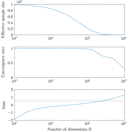
The upper subplot shows the estimated effective sample size. By D=512 importance weighted 100000 draws have only a few practically non-zero weights. The middle subplot shows the convergence rate compared to independent sampling, ie, how fast the variance goes down. By D=1024 the convergence rate has dramatically dropped and getting any improvement in the accuracy requires more and more draws. The bottom subplot shows Pareto khat diagnostic (see the paper for details). Dashed line is k=0.5, which the limit for variance being finite and dotted line is our suggestion for practically useful performance when using PSIS. But how can khat be larger than 0.5 when we have bounded weights! Central limit theorem has not failed here, but we have just not reach yet the asymptotic regime to get CLT to kick in!
The next plot shows more information what happens with D=1024.
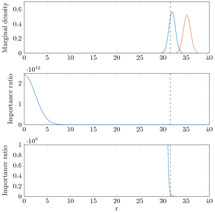
Since humans are lousy in looking at 1024 dimensional plots the top subplot shows the 1 dimensional marginal density of the target (blue) and the proposal (red) densities of the distance from the origo r=sqrt(sum_{d=1}^D x_d^2). The proposal density has only 1.1 larger scale than the target, but most of the draws from the proposal are away from the typical set of the target! The vertical dashed line shows 1e-6 quantile of the proposal, ie when we draw 100000 draws, 90% of time we don’t get any draws from there. The middle subplot shows the importance ratio function, and we can see that the highest value is at 0, but that value is larger than 2*10^42! That’s a big number. The bottom subplot scales the y axis show that we see importance ratios near that 1e-6 quantile. Check the y-axis: it’s still from 0 to 1e6. So if we are lucky we may get a draw below the dashed line, but then it’s likely to get all the weight. The importance function is practically as steep everywhere where we can get draws in a time of the age of the universe. 1e-80 quantile is at 21.5 (1e80 is the estimated number of atoms in the visible universe). and it’s still far away from the region where the boundedness of the importance ratio function starts to affect.
I have more similar plots with thick tailed Student’s t, mixture of proposals etc, but I’ll save you from more plots. As long as there is some difference in target and proposal taking the number of dimensions to high enough, IS and PSIS break (PSIS giving slight improvement in the performance, and more importantly can diagnose the problem and improves the Monte Carlo estimate).
In addition that we need to take into account that many methods which work in small dimensions can break in high dimensions, we need to focus more on finite case performance. As seen here it doesn’t help us that CLT holds if we never can reach that asymptotic regime (same as why Metropolis algorithm in high dimensions may require close to infinite time to produce useful results). Pareto diagnostics has been empirically shown to provide very good finite case convergence rate estimates which also match some theoretical bounds.
PS. There has been lot of discussion in comments about typical set vs. high probability set. In the end Carlos Ungil wrote
Your blog post seems to work equally well if you change
“most of the draws from the proposal are away from the typical set of the target!”
to
“most of the draws from the proposal are away from the high probability region of the target!”
I disagree with this, and to show evidence for this I add here couple more plots I didn’t include before (I hope that this blog post will not have eventually as many plots as the PSIS paper).
If the target is multivariate normal, we get bounded weights by using Student-t distribution with finite degrees of freedom nu, even if the scale of the Student-t is smaller than the scale of the target distribution. In the next example the target is same as above, and the proposal distribution is multivariate Student-t with degrees of freedom nu=7 and variance=1.
The following figure shows when the number of dimensions go from 1 to 1024.
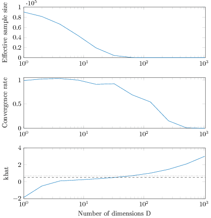
The upper subplot shows the estimated effective sample size. By D=64 importance weighted 100000 draws have only a few practically non-zero weights. The middle subplot shows the convergence rate compared to independent sampling, ie, how fast the variance goes down. By D=256 the convergence rate has dramatically dropped and getting any improvement in the accuracy requires more and more draws. The bottom subplot shows Pareto khat diagnostic which predicts well the finite case convergence rate (even if asymptotically with bounded ratios k<1/2).
The next plot shows more information what happens with D=512.
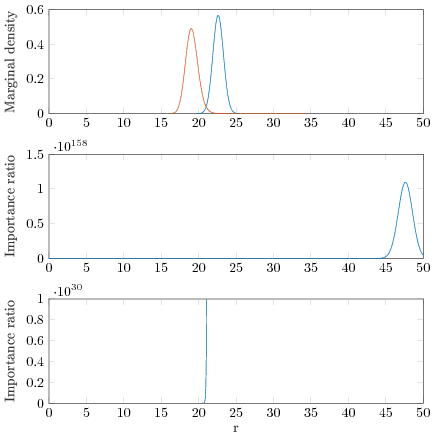
The top subplot shows the 1 dimensional marginal density of the target (blue) and the proposal (red) densities of the distance from the origo r=sqrt(sum_{d=1}^D x_d^2). The proposal density has the same variance but thicker tail. Most of the draws from the proposal are away from the typical set of the target and in this towards higher densities than the density in the typical set. The middle subplot shows the importance ratio function, and we can see that the highest value is close to 47.5 and then the ratio function starts to decrease again. The highest value of the ratio function is larger than 10^158. The region with highest value is far away from the typical set of the proposal distribution. The bottom subplot scales the y axis show that we see importance ratios near the proposal and the target distributions. The importance ratio goes from very small values up to 10^30 in very narrow range, and thus it’s likely that the largest draw from the proposal will get all the weight. It’s unlikely that in practical time we would get enough draws to get the asymptotic benefits of bounded ratios to kick in.
PPS. The purpose of this post was to illustrate that bounded ratios and asymptotic convergence results are not enough for the practically useful performance for IS, but there are also special cases where due to special structure of the posterior we can get practically good performance with IS, and especially with PSIS, also in high dimensions cases (PSIS paper has 400 dimensional example with khat<0.7).
> most of the draws from the proposal are away from the typical set of the target!
How are you defining typical set here?
Intuitively, it’s where random samples from the posterior will land. The discrete case is covered in the Wikipedia page:
https://en.wikipedia.org/wiki/Typical_set
Cover and Thomas’s book cover the continuous case with differential entropy. I cover the basic idea in my case study with examples (borrowed from McKay’s great info theory book, which is also available free online in PDF form with permission of the publisher):
http://mc-stan.org/users/documentation/case-studies/curse-dims.html
Hi Bob,
I asked because I was one of the people who felt your informal usage of typical set was incorrect in the technical sense. See also our discussion on your blog post
For example, why not just say ‘high probability set’? Or do you actually mean ‘typical set’? If so, why the typical set and not the high probability set?
I’m not an expert on typical sets and high probability sets, but inspired by this question I wanted to learn what is the difference between these. I didn’t yet find an answer in continuous case, but with a quick google search I found this http://mat.hjg.com.ar/tic/img/lecture4.pdf, which says
If the sequence is very long (ie X_i is high dimensional) it would be very unlikely to observe sequence of all 1s even if it is the single most probable sequence. In continuous case in high dimensions it’s unlikely we observe anything near the mode. So it seems typical set is more appropriate term.
If you have a better reference for typical set vs high probability set, please post in a comment.
Bob’s references, in particular Cover and Thomas and Mackay are fine, and discuss the difference. The high probability set (of level alpha) is simple to define: the smallest set containing at least alpha of probability. The typical set is more convoluted and relies on the AEP to make sense of imo.
I think the comparison you give is somewhat misleading: you are comparing a single realisation to a set of realisations. The same argument can be made against any other single observation, however this would be even more unlikely than the mode point (in the continuous case all points have zero probability anyway, but let’s consider the discrete case for concreteness).
By definition any single observation has a higher probability of landing in the high probability set than in the typical set, though the difference is asymptotically negligible, as shown by the AEP.
The most convincing argument for the typical set that I can think of is essentially the same as that given by Mackay: it is a convenient approximation to the high probability set.
Which is fine, but this undermines the selling point of the ‘counterintuitiveness’ of the typical set vs the high probability set. The mode is in the high probability set and so isn’t inherently ‘bad’ as seems to be the implication of some of Bob’s posts etc. It’s just that one can throw out the mode point and still get a set of approximately alpha of probability.
You can also throw out any other point and still get a set of approximately alpha of probability – in fact you will get one of (very slightly) higher probability.
My view on this is that typical set is good because:
– it’s common English meaning is useful to people who don’t know information theory
– it is the set we want (or very close to it)
– it’s definition actually matches what we want (actually for LOO we want that the log of a nonlinear function of the sample converges to almost the right thing, but this is “close enough)
– it emphasises the link between the typical set and the small set you need for geometric ergodic. Intuitively they’re complements.
You’re argument appears to be that you think we’re not using the technical definition. I don’t agree with you. If your problem is communication, I really think typical set is unambiguous to both technical and non-technical communities.
> it’s common English meaning
What’s wrong with ‘high probability set’?
> it is the set we want (or very close to it)
What’s wrong with ‘high probability set’?
> it’s definition actually matches what we want
What’s wrong with ‘high probability set’?
etc.
Or do you actually want “a set of sequences whose probability is close to two raised to the negative power of the entropy of their source distribution”? I.e. the typical set?
I’m not sure why you think repeating your self is making your point better. I prefer typical set for the reasons set out above.
> What’s wrong with ‘high probability set’?
Recently I read a footnote (https://www.aqr.com/cliffs-perspective/wild-but-not-crazy) giving the following reason for the use of continuously compounded returns: “They are a bit better behaved than simple compound returns. Plus, I always feel smarter using logs.”
In the “typical set” vs “high probability set” choice I still don’t get what is the objective reason for preferring the former, given that in practice the refer to the same set.
Carlos: I’m glad you comment around here!
Dan – when I feel people don’t address my question clearly I’m not sure what else to do but ask it again. I think I’ll give up on arguing with the Stan folk about this, as the typical responses seem unhelpful with high probability
If you don’t want to use “typical set”, don’t. I don’t like using the word “cognisant” because I prefer a synonym. I don’t feel the urge to interrogate people as to why they use it.
Ojm: I literally gave you four reasons (the last two very specifically using the technical definition). I’m done with this now.
ojm, Carlos: i’m glad you both stick around..
ojm: I think it’s an interesting fact that essentially all of the probability mass in a high dimensional posterior is in the set where log(p(x)) is within epsilon of some special value lp*
If we just *define* the word “typical set” to mean “the set of x values such that log(p(x)) = lp* +- epsilon”
and we define the high probability mass (HPM) set to mean “the smallest set such that integrate(p(x)) = 1-alpha”
then it’s an interesting fact that the two sets both have basically all of the probability mass in them. It seems the main difference between them is “on the boundary” where the HPM set includes the mode, and the typical set doesn’t include the mode and as a consequence includes a negligibly wider bit of the “tail” than the HPM set.
From a practical perspective it seems to me that arguing over these two is like arguing whether we should include a particular hair on your head, and a particular sliver of your fingernail as “part of your body”. Some people prefer including the head and leaving out the sliver of fingernail, some people prefer to include the fingernail, and leave out some of the hair… either way almost every portion of your body is included, so for people who want to calculate the mass of your liver or the volume of your blood or other “functionals of the set” they get the same answer regardless.
ojm: my biggest problem is that the *usual* definition of typical set is about *sequences* of independent draws from a single univariate generating process (thereby producing a high dimensional product space). However in Stan/Bayes we’re interested in *points from a high dimensional probability space* which are not sequences of independent draws from a univariate generator. The fact about the log(p(x)) still being nearly constant is what now defines the subset of the space… so when you look up in wikipedia or elsewhere, it’s hard to map technical definitions as used in info theory to technical definitions as used by say Bob Carpenter in his case studies.
One “solution” to this communication problem would be to explicitly define the technical definition of the word “typical set” being used in the case studies.
DL – true, it is splitting hairs somewhat. But aomw arguments seem to be based on this hair split. For example the Stan folk consistently maintain that they are in fact interested in the typical set rather than the high probability set. So it seems worth examining.
ojm: If we want to get into the hair-split, the first thing we need is a proper definition of the typical set that applies to sampling from a high dimensional Bayesian posterior rather than from *sequences of independent draws from univariate distributions*. The sequences definition is very useful in information theory because there we are talking about communication across a channel… a sequence of symbols is how we communicate information.
In the Stan case, it’s very easy to see, practically speaking, that once the HMC process has settled into stationarity, all the samples are within epsilon of having the same value for log(p(x)). Basically, all the probability mass is in this constant lp region. It’s also all in the HPM region as well, it’s just that these sets overlap on a set of nearly measure 1, and the regions where they don’t overlap has very very small total measure, either because the volume is small (near the mode), or the density falls off dramatically quickly (towards the “tail”).
It seems to me that the reason the Stan crew focuses on the typical set (as defined by near constant log(p)) is that log(p(x)) is something they’re calculating all the time, and the samples all have nearly the same value, and this just happens because of the geometry of high dimensions, not because they have to “avoid” the mode intentionally. When you’re calculating a thing all the time, and using it to determine whether your algorithm is working properly, it’s more obvious to focus on that aspect.
Basically, if you see a bunch of samples that come from a region with dramatically different log(p(x)) it’s an indicator that either you haven’t converged to stationarity of the sampler, or there’s a bug in the code. You shouldn’t ever see a sample near the mode, simply because the volume of the region near the mode is so small you effectively can’t hit it, because you’re starting each iteration with a random velocity vector. Similarly, you shouldn’t see samples with lp much less (more negative) than the typical set value because even though the volume of space with values like that is effectively infinite, the “energy” required to get there is prohibitively large.
So, I think the fact that nearly all the probability mass is in the typical set, combined with the fact that Stan explicitly calculates log(p(x)) at every iteration and spits it out in the output… and the fact that naturally through correct sampling, in high dimensions, essentially every sample has a constant value for log(p(x))… leads to a focus on that set. Rather than any other fundamental reason.
DL – yeah maybe man. If so I dunno why they don’t just say so though. I’m probably missing something here but I doubt I’m going get anywhere with discussing the nuances here.
+1 (to Daniel Lakeland’s comments). Also, I think what Bob said is also easy to lose sight of: “intuitively, it’s where random samples from the posterior will land” (that is, think about this *generatively*).
Daniel: yep. That’s basically exactly it (at least from my viewpoint. The Stan team is far from homogeneous and literally no one on earth has ever wanted met to speak for them). Nice explanation.
ojm: I really think this is it, because when you’re using Stan and/or debugging Stan models, the near-constancy of the lp variable and traceplots of lp are extremely useful for figuring out how well Stan is doing at sampling. You know it’s not working if lp is still trending or oscillating or stuck somewhere and not changing at all.
But from a theoretical perspective, I agree with you that the mode is not “to be avoided” it’s just not very helpful for calculating expectations, because there’s a LOT of mass elsewhere you need to take into account to get good expectation calculations.
> If the sequence is very long (ie X_i is high dimensional) it would be very unlikely to observe sequence of all 1s even if it is the single most probable sequence. In continuous case in high dimensions it’s unlikely we observe anything near the mode. So it seems typical set is more appropriate term.
It is even more unlikely that we observe anything near any other given point.
When we look a a sequence of 0/1 bits from a one-dimensional binomial distribution, the concept of a typical sequence may be interesting because the permutations are interchangeable. For example, we are often interested in the proportion of 1s and 0s.
When we look at a single realization of a highly-dimensional distribution (corresponding to coordinates in the sample space) what sense does the idea of a typical sequence make? Unless all the coordinates are independently sampled from the same distribution, we cannot say that they are a sequence of realizations of a variable.
And even if we accept that the coordinates form some kind of sequence, the permutation of coordinates results in “similar” points only if the problem (probability distribution and function of interest) has spherical symmetry. If we calculate the expected value of an arbitrary function f(x1,..,x1000) for 1000-dimensional normal distribution two points in the typical set are in no meaningful way closer to each other than they are close to the origin.
Based on the discussion here I think I have understood distinction between typical set and high probability set (at least approximately correctly) correctly, but let’s check that.
ojm wrote
Important part of my blog post was that in order to get in the asymptotic regime of bounded ratio benefits requires that we get draws from the proposal distribution which are close to the the mode. Close to the mode being maybe inside sphere with radius 5. I mentioned that probability mass close to the mode inside a sphere with radius approximately 21.5 is less than one per the number of atoms in the observable universe. For me it seems unlikely that with current computers we would get draws inside this sphere (r approx 21.5) in my lifetime so I would call that untypical set. If high probability set includes (in probability, epsilon etc.) inside of that sphere (r approx 21.5) and typical set does not include inside of that sphere (r approx 21.5) then I think typical set is more useful for me to describe what happens in finite case. For the theoretical (but completely impractical) asymptotic case I might be fine with high probability set, too.
Pick a set of fixed volume. Then the high probability set is the one of that volume that you are most likely to see in your lifetime. When you compare sets of different volume then the comparison is not ‘fair’ so to speak. If there was no radial symmetry then would you lump all points of a fixed radius away together?
If we pick a set of fixed volume large enough that its total probability is not negligible, then the high probability set with that volume will overlap the typical set, and if we sample until we hit this volume, the sample point will probably be in the typical set “portion” of this set just because the total fraction of the volume that is in the typical st portion is so much larger than the fraction that is near the mode.
In high dimensions, the HP set is basically equal to the typical set, plus a tiny volume near the mode, minus a miniscule wafer thin shell away from the mode. The euclidean distance to the mode from any point in the typical set can be quite large, and yet it doesn’t matter because the volume near the mode is so small, we can go “deep” into this “Modal tail” without adding much probability, hence we only need to shave a razor thin shell off the “outside”
If you think a bit generatively – about drawing samples from the posterior distribution – it is clear that in high dimensions you will never draw samples near the mode. As you say, this is not due to any deliberate “modal exclusion”. Thus, algorithms to use MCMC to draw posterior samples (or compute expectations wrt posterior, as some say), should be guided by geometric information that aids in discovering the ‘typical set’, rather than this ‘HP set’, although their overlap is quite substantial.
DL – yes, I agree. But note also that by talking about points in a shell a given distance away you are talking about a set.
As soon as you go to the second part of what you are saying you are dropping the constraint of comparing sets of fixed volume. Whenever you fix either total probability or volume, the high probability set is natural. Every argument for the typical set after this drops the fixed constraint and hence makes comparisons somewhat arbitrary. I would like to see a single example where the volume or probability is held fixed that makes the typical set more natural.
Of course the volume of a shell of given radius is larger in high dimensions than the small ball around the mode. But that’s not the point. (This is where eg Bob jumps in and says ‘that’s the point’ – but no, it is not my point.
Then Dan jumps in and says ‘well what is your point?’. Then I say something snarky and we unfollow each other on Twitter, and all is well with the world).
I will buy you a beer and we can chat some day if we’re ever in the same place, but the internet is clearly not a medium that we can successfully communicate on.
Agreed :-)
Or, how about an example without spherical symmetry? The symmetry makes it natural to think about the shell as ‘one thing’. But if you compare a small fixed segment of the shell to a volume around the mode of the same volume then the points are more likely to land around the mode than in the given segment, ie in the portion of the high probability set not the portion of the typical set.
ojm, well what IS your point? :) In the bigger sense, isn’t the point to evaluate probability measures (requiring integration of densities over volumes)?
It all started with: http://statmodeling.stat.columbia.edu/2017/03/15/ensemble-methods-doomed-fail-high-dimensions/
Where it is stated
> Why ensemble methods fail: Executive summary
1. We want to draw a sample from the typical set
2. The typical set is a thin shell a fixed radius from the mode in a multivariate normal
3. Interpolating or extrapolating two points in this shell is unlikely to fall in this shell
4. The only steps that get accepted will be near one of the starting points
5. The samplers devolve to a random walk with poorly biased choice of direction
Without disagreeing with 2-5, I question the premise 1.
I think one reason I push back is a sense (there and elsewhere) of an emphasis on ‘wow counterintuitive result – the mode is bad’. But this is not so counterintuitive in the sense that the mode is no worse than any other single point. If the mode is included the appropriate number of times, along with other points being included an appropriate number of times, it’s fine. So it seems disingenuous to use that as premise one in criticisms of other methods – even if there are completely legitimate other criticisms to make!
I think the pushback plays a role too – if people just said ‘yeah we want the high probability set but the typical set is convenient for us’ then cool. But when people actually try to make the argument that we really truly want the typical set and not the high probability set, I dunno, I guess it just provokes me to pointlessly argue on the internet about it.
“If the mode is included the appropriate number of times, along with other points being included an appropriate number of times, it’s fine.”
But, due to the probability mass in the vicinity of the mode being nearly zero, the appropriate number of times to sample near the mode in any reasonable sample size… like thousands to millions of samples… is *zero*
whereas the appropriate number of times to have samples whose log(p(x)) = lp* is basically N, the number of samples you’re drawing. Sure, any *given* point in the typical set shouldn’t appear, but the fraction of points which are in the typical set should be essentially all of them.
> the fraction of points which are in the typical set should be essentially all of them.
The fraction of points which are in the high density region is also esentially all of them, so if there is a good reason to prefer the typical set it may be somewhere else :-)
“The fraction of points which are in the high density region is also esentially all of them”
No, that’s not true. In the spherical symmetry normal distribution case, the highest density region is the mode near x=0, let’s say with radius 1 or so, but in a 1000 dimensional normal, the radius of such randomly selected points has a chi distribution with 1000 degrees of freedom and in such a distribution 99% of the points are outside radius 30 or so.
so points are not near the “high density” region, but they are in the “high probability” region because the “high probability” region includes everything from radius 0 to radius say 36, however almost all the points are radius 30-36 not anywhere “near” radius 0
I use High Density Region and High Probability Region as synonyms: the region where the probability density function is above some threshold. For a fixed volume or probability mass, what difference do you see between the HDR and the HPR?
Carlos, take the 1000 dimensional unit normal. I do
vec = rnorm(1000)
sum(sapply(vec,function(x),dnorm(x,log=TRUE)))
and get
-1411.434
and sqrt(sum(vec*vec)) = 31.38
now I investigate the density near the mode:
I do sum(sapply(rep(0,1000),function(x) dnorm(x,log=TRUE)))
and get
-918.9385
so the density near my randomly chosen point, which is in the typical set, is exp(-492.5) times less dense than the density near the mode. So I don’t see how we can call that a high *density*
On the other hand, the probability, which involves integrating density * volume is very large for shells of radius 30-35 because the volume of those shells is enormous, not because the density is anything much more than 0 to 200 decimal places.
Daniel, what is the 95% HDR in your example?
The usual sense of 95% region (trimming on both ends) we can get by
sqrt(qchisq(.125,1000)), sqrt(qchisq(.975,1000))
which is the shells for radius between 30.8 and 33.008
But ojm’s set, is the ball of radius less than
sqrt(qchisq(.95,1000)) = 32.7823
so includes the whole region from radius 0 to 32.7823 and this volume is slightly smaller than the volume between 30.8 and 33.008
but in both cases, almost all the points are in the range r = 31 to 32 and essentially none of the points are inside radius 28
sqrt(qchisq(1e-6,1000))
[1] 28.31297
The HD in “95% HDR” means that the points within the region have higher probability density than the points without the region.
The 95% HDR *is* the ball of radius 32.8 (assuming your calculation is correct).
The 95% HDR *is not* the shell between 30.8 and 33.0 (obviously, because the probability density is higher for the points in the inner “hole” than for the points in the shell).
without the region => outside the region
Ok, fine ojm’s set and your “95 HDR” are both the ball of radius less than 32.8 but note that this is predicated on *both* high density *and* high total probability not just “the region where the probability density function is above some threshold”
If we took the region where probability density in the 1000 dimensional space is above say 0.001 times the peak density… which is a pure density based definition of a set, then this set is the ball of radius less than around 3.7
and this ball is inside your 95% High Probability ball around 0 but *does not intersect the typical set*, and this ball has essentially zero points in it precisely because it doesn’t intersect the typical set.
my calculation:
dnorm(3.7)/dnorm(0)
[1] 0.001064766
pchisq(3.7^2,1000,log.p=TRUE)
[1] -1656.402
so the total probability inside the set of density greater than 0.001 fraction of the peak density is exp(-1656)
> this is predicated on *both* high density
That’s the HD.
> *and* high total probability
That’s the 95%.
> not just “the region where the probability density function is above some threshold”.
More precisely the region where the probability density function is higher than the threshold that makes the probability mass contained in the region 95%.
I’m not sure what do you find so dificult about the concept of the HDR. It is the natural extension of the one-dimensional HDI. I’m sure you know and understand HPD intervals (the shortest credible intervals). How is this different?
In 1000 dimensions the *geometry* of the HDR is very weird. In the unit normal case we can get a little intuition, but in the general case, it’s like trying to describe the surface of a human brain or something.
I do fully understand when you say the 95% HDR region you are talking about what I and OJM were calling the High Probability region. I guess the point is that when you use the “typical set” or you use the 95% HDR region, essentially all the points are *in both* and so the distinction is mainly occurring in regions that actually don’t matter, like in my example the radius less than 3.7 ball…
In the more general high dimensional posterior geometry, defining the 95%HDR region as “the smallest volume set containing 95% of the probability” is fine, but constructing it is basically impossible, in other words, you can’t compute with it…. But you *can* compute with the typical set because it’s the “set where density is essentially constant and equal to exp(lp*)+-epsilon for some particular lp* and epsilon sufficient to get you 95% of the mass.
HMC naturally is attracted to this set because it does correct unbiased sampling, and essentially all the samples are in this set (which is typically near the boundary of the 95%HPD set)
> HMC naturally is attracted to this set because it does correct unbiased sampling, and essentially all the samples are in this set
It will also be naturally attracted to the HPD set, for the same reason. Actually it will be slightly more attracted to the HPD set, given than it is slightly more compact than the typical set (for the same probability mass).
> (which is typically near the boundary of the 95%HPD set)
In high dimensions, the whole HPD set is also near its boundary.
“set where density is essentially constant”
*constant* as in “ranging over ~35 orders of magnitude” (for the 95% set in the 1000-dimensional standard gaussian).
“As soon as you go to the second part of what you are saying you are dropping the constraint of comparing sets of fixed volume”
I wasn’t intending that. Suppose we start with the typical set and it’s volume is V.
Now, we want to compare it to the high probability set of *equal volume*. Let’s also just for ease of discussion stick to the independent symmetric normal…
So, the typical set is basically a shell at radius r with half-width w.
The high probability set is the entire ball within radius r+w-epsilon where we choose epsilon so that now the volume we added inside the ball is removed from the exterior “skin” retaining the constant volume V. epsilon is a *very small* number because there is almost no volume inside the ball.
Now the two sets have the same volume by construction, the total probability is basically 1 for both of them to zeroth order, but to first order, the HP set has an epsilon of higher probability. Still, if we randomly sprinkle points inside the HP set according to the probability mass, *essentially all of those points are in the portion of the HP set that intersects the original Typical Set*
If we take the sprinkled points and select from them uniformly at random, with a reasonable finite sample size, say N=100000 then *every one of them will be in the Typical Set portion* virtually guaranteed.
So if we have an algorithm that tends to bias us towards moving in the direction of the mode, to get a correct sample we need to actually *undo this bias* or we will over-sample the mode.
> If we take the sprinkled points and select from them uniformly at random, with a reasonable finite sample size, say N=100000 then *every one of them will be in the Typical Set portion* virtually guaranteed.
Every one of them will be also in the High Density Region portion, virtually guaranteed. And if you calculate how many points can you expect to miss (which we agree will be a very small quantity), the typical set will get worse coverage than the HDR by construction.
> So if we have an algorithm that tends to bias us towards moving in the direction of the mode, to get a correct sample we need to actually *undo this bias* or we will over-sample the mode.
If we had an algorithm that tended to bias us towards moving far from the mode we would also need to undo that bias to get a correct sample. Using unbiased algorithms is probably better :-)
“If we had an algorithm that tended to bias us towards moving far from the mode we would also need to undo that bias to get a correct sample.”
Yes, but the point of the original post that brought ojms concern to the forefront was that people were proposing algorithms such as sampling along a line between two points which did bias things towards moving outside the typical set (and in the unit normal high dim case, towards the mode), and the metropolis hastings correction required to get unbiased samples caused the algorithms to devolve to tiny-step-size diffusions along the “surfaces” defined by the typical set, and hence they were unhelpful.
> algorithms such as sampling along a line between two points which did bias things towards moving outside the typical set (and in the unit normal high dim case, towards the mode)
Are you sure this bias exists? As the number of dimensions increases, the probability that the segment connecting two random points from a hypersphere passes near the origin vanishes.
Carlos: I wasn’t the one who posted that, it was Bob who did the case study, so no I’m not sure the bias exists, but I can say that it doesn’t have to pass near the origin to go into useless territory, it just needs to deviate off the razor thin curved shell. Basically, if you take any two points on an eggshell and you draw a line between them what’s the probability that a randomly chosen point on the line will be inside the material of the calcified eggshell? If the points are very close together then it works ok. But if they’re far apart essentially none of the points are inside the eggshell material. If you can take a sequence of points that are close together and continue to travel in a consistent direction, you get a trajectory along the eggshell, if you are constantly changing directions, you get a random walk on the eggshell, and you never go very far.
In practice, fitting models in Stan, my complicated models often need very small timesteps and this is because they have to follow a complicated curved “surface” in N dimensions, a directed trajectory “along the eggshell”
The “algorithm” that was shown to fail (taking the median from two random points from the distribution) was a straw man. It’s quite obvious that it’s going to result in a more concentrated distribution and there is no need to go beyond one or two dimensions to realize that. Now we can discuss how in high dimensions the problem gets worse, but that’s completely irrelevant because the algorithm was never supossed to work.
The funny thing is that if you have a multi-dimensional standard normal distribution the median of two random points is distributed as a multi-dimensional normal distribution of variance 1/2. Therefore, it’s enough to modify the algorithm slightly from (a+b)/2 to (a+b)/sqrt(2) to fix the problem (whatever the number of dimensions).
Maybe ensemble algorithms have issues, but I don’t think that blog post provided any indication of it.
Your blog post seems to work equally well if you change
“most of the draws from the proposal are away from the typical set of the target!”
to
“most of the draws from the proposal are away from the high probability region of the target!”
No. We can also have a such proposal distribution (e.g. Student-t with nu=7, variance=1) that we have bounded ratios and “most of the draws from the proposal are *towards* to the high probability region of the target” and still have “most of the draws from the proposal are away from the typical set of the target”. This is illustrated in the one of the plots I left out, but I can add it later today.
Of course my comment was about what you wrote, not about other things you could have written.
For the case considered in your PS the problem is also easy to see in terms of high density regions. The HDR for the proposal covers only a small part of the HDR for the target so it is not surprising that importance sampling behaves badly.
> For the case considered in your PS the problem is also easy to see in terms of high density regions. The HDR for the proposal covers only a small part of the HDR for the target so it is not surprising that importance sampling behaves badly.
But this holds only for the second example, but not in the first example.
The point I was trying to make isn’t that we need to exclude the mode in some way. It’s just that a lot of people develop intuitions for algorithms based on one or two dimensional examples where there’s a lot of volume around the mode. They think the point is to try to find a mode and sample near there. That won’t actually work, because if you take draws near the mode, estimates like posterior variances are going to be wrong. The point is to take draws that let you estimate the expectations you care about.
Of course, the sense in which the mode is excluded from the typical set is also relevant—its log density is atypically high. If you take lots of draws from the posterior, their log density will be bounded pretty far away from the mode’s log density. Again, nothing needs to exclude the mode—draws near it in log density just don’t come up.
What if your target functional is the maximum log probability? Will sampling from the typical set be good for this?
ojm, next time you run a Stan model, you might have a look at the pairs() plot. You can examine lp_, etc. no problem, if that is what you are after here.
Sampling won’t get you max log prob, because with sampling you will never see the mode, it’s just a fact about probability. You need optimization for this.
Daniel, you will see the mode of the posterior for the marginal parameter distributions though…
If you want a max posterior mode you need to use an optimizer. It’s why Stan has both sampling and optimization built in.
Bayesians don’t do optimization when it can be avoided. What we care about for Bayesian inference is posterior expectations. For example, point estimates are typically calculated as posterior means, because that minimizes expected squared error (relative to the model, of course); poserior median minimizes expected absolute error. The posterior mode doesn’t have any such properties. So we don’t pay much attention to the mode.
Having said that, Andrew likes to think of a Laplace approximation on the unconstrained scale as a kind of approximate Bayesian posterior. That makes it very much like variational inference, which drops an approximate distribution on an approximate posterior mean rather than posterior mode.
I would think my comments are impossible to understand if it wasn’t for Carlos…
I think it comes down to this: if you want to approximate an independent identically distributed sample from a high dimensional posterior distribution, the best available algorithm is Stan’s version of HMC. That algorithm samples in the region where you’d find your samples if they were IID and that region is roughly the region where log(p(x)) is near-constant and equal to some value that is much lower than the value at the mode.
so, either IID sampling, or HMC sampling will both give you points that are in the typical set and *not* particularly near the mode in euclidean distance.
If you want something that can’t be calculated effectively by IID sampling, such as the location of the mode, then you also won’t be able to calculate it effectively with HMC type sampling.
The point of HMC sampling is that it gives you a sample which is “close to IID” in the sense of effective sample size is nearly the same as the actual sample size. Anything you can calculate with IID samples you can calculate pretty well with HMC samples…
ojm, what Daniel and Bob said is definitely technically correct, but it feels like you are trying to ask something else. My comment was only tangentially related in that I am pointing out for any marginal of interest, sampling from the typical set definitely does enable one to visually find the mode…